作业二
作业内容:
在本作业中,你将练习编写反向传播代码,训练神经网络和卷积神经网络
超参数调试
深度学习可能存在的参数

其中学习速率是需要调试的最重要的超参数。
如何选择调试值呢?
在早一代的机器学习算法中,如果你有两个超参数,这里我会称之为超参1,超参2,常见的做法是在网格中取样点,像这样,然后系统的研究这些数值。,实践证明,网格可以是5×5,也可多可少,但对于这个例子,你可以尝试这所有的25个点,然后选择哪个参数效果最好。当参数的数量相对较少时,这个方法很实用。
在深度学习领域,我们常做的,我推荐你采用下面的做法,随机选择点,所以你可以选择同等数量的点,对吗?25个点,接着,用这些随机取的点试验超参数的效果。之所以这么做是因为,对于你要解决的问题而言,你很难提前知道哪个超参数最重要,正如你之前看到的,一些超参数的确要比其它的更重要。
为超参数选择合适的范围
假设你要选取隐藏单元的数量,假设,你选取的取值范围是从50到100中某点,这种情况下,看到这条从50-100的数轴,你可以随机在其取点,这是一个搜索特定超参数的很直观的方式。或者,如果你要选取神经网络的层数,我们称之为字母L,你也许会选择层数为2到4中的某个值,接着顺着2,3,4随机均匀取样才比较合理,你还可以应用网格搜索,你会觉得2,3,4,这三个数值是合理的,这是在几个在你考虑范围内随机均匀取值的例子,这些取值还蛮合理的,但对某些超参数而言不适用。
看看这个例子,假设你在搜索超参数(学习速率),假设你怀疑其值最小是0.0001或最大是1。如果你画一条从0.0001到1的数轴,沿其随机均匀取值,那90%的数值将会落在0.1到1之间,结果就是,在0.1到1之间,应用了90%的资源,而在0.0001到0.1之间,只有10%的搜索资源,这看上去不太对。
反而,用对数标尺搜索超参数的方式会更合理,因此这里不使用线性轴,分别依次取0.0001,0.001,0.01,0.1,1,在对数轴上均匀随机取点,这样,在0.0001到0.001之间,就会有更多的搜索资源可用,还有在0.001到0.01之间等等。
最后,另一个棘手的例子是给B取值,用于计算指数的加权平均值。假设你认为是0.9到0.999之间的某个值,也许这就是你想搜索的范围。记住这一点,当计算指数的加权平均值时,取0.9就像在10个值中计算平均值,有点类似于计算10天的温度平均值,而取0.999就是在1000个值中取平均。
如何搜索超参数
我见过大概两种重要的思想流派或人们通常采用的两种重要但不同的方式。
一种是你照看一个模型,通常是有庞大的数据组,但没有许多计算资源或足够的CPU和GPU的前提下,基本而言,你只可以一次负担起试验一个模型或一小批模型,在这种情况下,即使当它在试验时,你也可以逐渐改良。比如,第0天,你将随机参数初始化,然后开始试验,然后你逐渐观察自己的学习曲线,也许是损失函数J,或者数据设置误差或其它的东西,在第1天内逐渐减少,那这一天末的时候,你可能会说,看,它学习得真不错。我试着增加一点学习速率,看看它会怎样,也许结果证明它做得更好,那是你第二天的表现。两天后,你会说,它依旧做得不错,也许我现在可以填充下Momentum或减少变量。然后进入第三天,每天,你都会观察它,不断调整你的参数。也许有一天,你会发现你的学习率太大了,所以你可能又回归之前的模型,像这样,但你可以说是在每天花时间照看此模型,即使是它在许多天或许多星期的试验过程中。所以这是一个人们照料一个模型的方法,观察它的表现,耐心地调试学习率,但那通常是因为你没有足够的计算能力,不能在同一时间试验大量模型时才采取的办法。
另一种方法则是同时试验多种模型,你设置了一些超参数,尽管让它自己运行,或者是一天甚至多天,然后你会获得像这样的学习曲线,这可以是损失函数J或实验误差或损失或数据误差的损失,但都是你曲线轨迹的度量。同时你可以开始一个有着不同超参数设定的不同模型,所以,你的第二个模型会生成一个不同的学习曲线,也许是像这样的一条(紫色曲线),我会说这条看起来更好些。与此同时,你可以试验第三种模型,等等。或者你可以同时平行试验许多不同的模型,橙色的线就是不同的模型。用这种方式你可以试验许多不同的参数设定,然后只是最后快速选择工作效果最好的那个。
代码
best_model = None
################################################################################
# TODO: Train the best FullyConnectedNet that you can on CIFAR-10. You might   #
# find batch/layer normalization and dropout useful. Store your best model in  #
# the best_model variable.                                                     #
################################################################################
# *****START OF YOUR CODE (DO NOT DELETE/MODIFY THIS LINE)*****

model = FullyConnectedNet([100, 100, 100, 100], dropout=0.5, normalization=None, weight_scale=5e-2, reg = 1e-1)
learning_rate = 1e-4
solver = Solver(model, small_data,
              num_epochs=10, batch_size=64,
              update_rule=update_rule,
              optim_config={
                'learning_rate': learning_rate
              },
              verbose=True)
solvers['adam'] = solver
solver.train()
best_model = model
正则化
深度学习可能存在过拟合问题——高方差,有两个解决方法,一个是正则化,另一个是准备更多的数据,这是非常可靠的方法,但你可能无法时时刻刻准备足够多的训练数据或者获取更多数据的成本很高,但正则化通常有助于避免过拟合或减少你的网络误差。
如果你怀疑神经网络过度拟合了数据,即存在高方差问题,那么最先想到的方法可能是正则化,另一个解决高方差的方法就是准备更多数据,这也是非常可靠的办法,但你可能无法时时准备足够多的训练数据,或者,获取更多数据的成本很高,但正则化有助于避免过度拟合,或者减少网络误差,下面我们就来讲讲正则化的作用原理。
L2正则化是最常见的正则化类型,你可能听说过L1正则化,如果用的是L1正则化,最终会是稀疏的,也就是说向量中有很多0。
为什么正则化有利于预防过拟合呢?
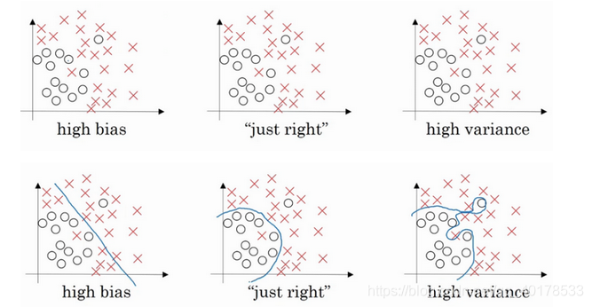
直观上理解就是如果正则化参数设置得足够大,权重矩阵W被设置为接近于0的值,直观理解就是把多隐藏单元的权重设为0,于是基本上消除了这些隐藏单元的许多影响。如果是这种情况,这个被大大简化了的神经网络会变成一个很小的网络,小到如同一个逻辑回归单元,可是深度却很大,它会使这个网络从过度拟合的状态更接近左图的高偏差状态。
但是会存在一个中间值,于是会有一个接近“Just Right”的中间状态。
直观理解就是参数增加到足够大,W会接近于0,实际上是不会发生这种情况的,我们尝试消除或至少减少许多隐藏单元的影响,最终这个网络会变得更简单,这个神经网络越来越接近逻辑回归,我们直觉上认为大量隐藏单元被完全消除了,其实不然,实际上是该神经网络的所有隐藏单元依然存在,但是它们的影响变得更小了。神经网络变得更简单了,貌似这样更不容易发生过拟合,不过在编程中执行正则化时,你实际看到一些方差减少的结果。
总结一下,如果正则化参数变得很大,参数W很小,z也会相对变小,此时忽略b的影响,z会相对变小,实际上,z的取值范围很小,这个激活函数,也就是曲线函数tanh会相对呈线性,整个神经网络会计算离线性函数近的值,这个线性函数非常简单,并不是一个极复杂的高度非线性函数,不会发生过拟合。
dropout 正则化
dropout正则化后为:
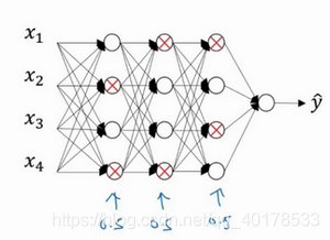
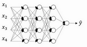
工作原理:假设你在训练上图这样的神经网络,它存在过拟合,这就是dropout所要处理的,我们复制这个神经网络,dropout会遍历网络的每一层,并设置消除神经网络中节点的概率。假设网络中的每一层,每个节点都以抛硬币的方式设置概率,每个节点得以保留和消除的概率都是0.5,设置完节点概率,我们会消除一些节点,然后删除掉从该节点进出的连线,最后得到一个节点更少,规模更小的网络,然后用backprop方法进行训练。
注意:在测试阶段不使用dropout函数
代码
def dropout_forward(x, dropout_param):
    """
    Performs the forward pass for (inverted) dropout.

    Inputs:
    - x: Input data, of any shape
    - dropout_param: A dictionary with the following keys:
      - p: Dropout parameter. We keep each neuron output with probability p.
      - mode: 'test' or 'train'. If the mode is train, then perform dropout;
        if the mode is test, then just return the input.
      - seed: Seed for the random number generator. Passing seed makes this
        function deterministic, which is needed for gradient checking but not
        in real networks.

    Outputs:
    - out: Array of the same shape as x.
    - cache: tuple (dropout_param, mask). In training mode, mask is the dropout
      mask that was used to multiply the input; in test mode, mask is None.

    NOTE: Please implement **inverted** dropout, not the vanilla version of dropout.
    See http://cs231n.github.io/neural-networks-2/#reg for more details.

    NOTE 2: Keep in mind that p is the probability of **keep** a neuron
    output; this might be contrary to some sources, where it is referred to
    as the probability of dropping a neuron output.
    """
    p, mode = dropout_param['p'], dropout_param['mode']
    if 'seed' in dropout_param:
        np.random.seed(dropout_param['seed'])

    mask = None
    out = None

    if mode == 'train':
        #######################################################################
        # TODO: Implement training phase forward pass for inverted dropout.   #
        # Store the dropout mask in the mask variable.                        #
        #######################################################################
        # *****START OF YOUR CODE (DO NOT DELETE/MODIFY THIS LINE)*****

        mask = np.ones((1, x.shape[1]))
        prop = np.random.rand(1, x.shape[1])
        mask[prop < p] = 0
        out = x*mask/p

        # *****END OF YOUR CODE (DO NOT DELETE/MODIFY THIS LINE)*****
        #######################################################################
        #                           END OF YOUR CODE                          #
        #######################################################################
    elif mode == 'test':
        #######################################################################
        # TODO: Implement the test phase forward pass for inverted dropout.   #
        #######################################################################
        # *****START OF YOUR CODE (DO NOT DELETE/MODIFY THIS LINE)*****

        out = x

        # *****END OF YOUR CODE (DO NOT DELETE/MODIFY THIS LINE)*****
        #######################################################################
        #                            END OF YOUR CODE                         #
        #######################################################################

    cache = (dropout_param, mask)
    out = out.astype(x.dtype, copy=False)

    return out, cache


def dropout_backward(dout, cache):
    """
    Perform the backward pass for (inverted) dropout.

    Inputs:
    - dout: Upstream derivatives, of any shape
    - cache: (dropout_param, mask) from dropout_forward.
    """
    dropout_param, mask = cache
    mode = dropout_param['mode']

    dx = None
    if mode == 'train':
        #######################################################################
        # TODO: Implement training phase backward pass for inverted dropout   #
        #######################################################################
        # *****START OF YOUR CODE (DO NOT DELETE/MODIFY THIS LINE)*****

        dx = dout*mask/dropout_param['p']

        # *****END OF YOUR CODE (DO NOT DELETE/MODIFY THIS LINE)*****
        #######################################################################
        #                          END OF YOUR CODE                           #
        #######################################################################
    elif mode == 'test':
        dx = dout
    return dx
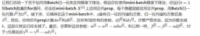
Batch归一化
深度学习文献中有一些争论,关于在激活函数之前是否应该归一化,或是否应该在应用激活函数后再规范值。实践中,经常做的是归一化激活前的值,这就是默认选择,那下面就是Batch归一化的使用方法。
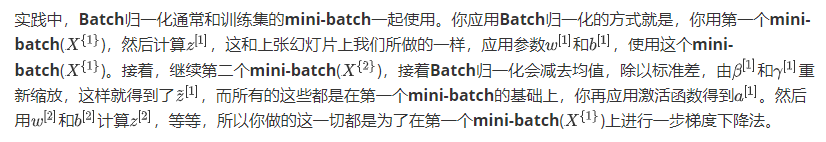
使用Batch归一化,你能够训练更深的网络,让你的学习算法运行速度更快。
代码
def batchnorm_forward(x, gamma, beta, bn_param):
    """
    Forward pass for batch normalization.

    During training the sample mean and (uncorrected) sample variance are
    computed from minibatch statistics and used to normalize the incoming data.
    During training we also keep an exponentially decaying running mean of the
    mean and variance of each feature, and these averages are used to normalize
    data at test-time.

    At each timestep we update the running averages for mean and variance using
    an exponential decay based on the momentum parameter:

    running_mean = momentum * running_mean + (1 - momentum) * sample_mean
    running_var = momentum * running_var + (1 - momentum) * sample_var

    Note that the batch normalization paper suggests a different test-time
    behavior: they compute sample mean and variance for each feature using a
    large number of training images rather than using a running average. For
    this implementation we have chosen to use running averages instead since
    they do not require an additional estimation step; the torch7
    implementation of batch normalization also uses running averages.

    Input:
    - x: Data of shape (N, D)
    - gamma: Scale parameter of shape (D,)
    - beta: Shift paremeter of shape (D,)
    - bn_param: Dictionary with the following keys:
      - mode: 'train' or 'test'; required
      - eps: Constant for numeric stability
      - momentum: Constant for running mean / variance.
      - running_mean: Array of shape (D,) giving running mean of features
      - running_var Array of shape (D,) giving running variance of features

    Returns a tuple of:
    - out: of shape (N, D)
    - cache: A tuple of values needed in the backward pass
    """
    mode = bn_param['mode']
    eps = bn_param.get('eps', 1e-5)
    momentum = bn_param.get('momentum', 0.9)

    N, D = x.shape
    running_mean = bn_param.get('running_mean', np.zeros(D, dtype=x.dtype))
    running_var = bn_param.get('running_var', np.zeros(D, dtype=x.dtype))

    out, cache = None, None
    if mode == 'train':
        #######################################################################
        # TODO: Implement the training-time forward pass for batch norm.      #
        # Use minibatch statistics to compute the mean and variance, use      #
        # these statistics to normalize the incoming data, and scale and      #
        # shift the normalized data using gamma and beta.                     #
        #                                                                     #
        # You should store the output in the variable out. Any intermediates  #
        # that you need for the backward pass should be stored in the cache   #
        # variable.                                                           #
        #                                                                     #
        # You should also use your computed sample mean and variance together #
        # with the momentum variable to update the running mean and running   #
        # variance, storing your result in the running_mean and running_var   #
        # variables.                                                          #
        #                                                                     #
        # Note that though you should be keeping track of the running         #
        # variance, you should normalize the data based on the standard       #
        # deviation (square root of variance) instead!                        #
        # Referencing the original paper (https://arxiv.org/abs/1502.03167)   #
        # might prove to be helpful.                                          #
        #######################################################################
        # *****START OF YOUR CODE (DO NOT DELETE/MODIFY THIS LINE)*****

        mean = np.mean(x, axis = 0, keepdims = True)
        var = np.var(x, axis = 0, keepdims = True)
        xnorm = (x - mean)/np.sqrt(var + eps)
        out = gamma*xnorm + beta
        running_mean = momentum*running_mean + (1 - momentum)*mean
        running_var = momentum*running_var + (1 - momentum)*var
        cache = [x, gamma, mean, var, eps]

        # *****END OF YOUR CODE (DO NOT DELETE/MODIFY THIS LINE)*****
        #######################################################################
        #                           END OF YOUR CODE                          #
        #######################################################################
    elif mode == 'test':
        #######################################################################
        # TODO: Implement the test-time forward pass for batch normalization. #
        # Use the running mean and variance to normalize the incoming data,   #
        # then scale and shift the normalized data using gamma and beta.      #
        # Store the result in the out variable.                               #
        #######################################################################
        # *****START OF YOUR CODE (DO NOT DELETE/MODIFY THIS LINE)*****

        x = (x - running_mean)/np.sqrt(running_var + eps)
        out = gamma*x + beta

        # *****END OF YOUR CODE (DO NOT DELETE/MODIFY THIS LINE)*****
        #######################################################################
        #                          END OF YOUR CODE                           #
        #######################################################################
    else:
        raise ValueError('Invalid forward batchnorm mode "%s"' % mode)

    # Store the updated running means back into bn_param
    bn_param['running_mean'] = running_mean
    bn_param['running_var'] = running_var

    return out, cache


def batchnorm_backward(dout, cache):
    """
    Backward pass for batch normalization.

    For this implementation, you should write out a computation graph for
    batch normalization on paper and propagate gradients backward through
    intermediate nodes.

    Inputs:
    - dout: Upstream derivatives, of shape (N, D)
    - cache: Variable of intermediates from batchnorm_forward.

    Returns a tuple of:
    - dx: Gradient with respect to inputs x, of shape (N, D)
    - dgamma: Gradient with respect to scale parameter gamma, of shape (D,)
    - dbeta: Gradient with respect to shift parameter beta, of shape (D,)
    """
    dx, dgamma, dbeta = None, None, None
    ###########################################################################
    # TODO: Implement the backward pass for batch normalization. Store the    #
    # results in the dx, dgamma, and dbeta variables.                         #
    # Referencing the original paper (https://arxiv.org/abs/1502.03167)       #
    # might prove to be helpful.                                              #
    ###########################################################################
    # *****START OF YOUR CODE (DO NOT DELETE/MODIFY THIS LINE)*****

    x, gamma, mean, var, eps = cache
    xnorm = (x - mean)/np.sqrt(var + eps)
    std = np.sqrt(var + eps)
    N, D = x.shape

    dbeta = np.sum(dout, axis = 0, keepdims = True)
    dgamma = np.sum(xnorm*dout, axis = 0, keepdims = True)
    dy = dout * gamma.reshape(1, -1)
    dx1 = dy/std
    dx2 = -np.sum(dy/(std*N), axis = 0, keepdims = True)
    dx3 = -np.sum(dy*xnorm/std**2, axis = 0, keepdims = True)*((x - mean)/N - np.sum(x - mean, axis = 0, keepdims = True)/N**2)
    dx = dx1 + dx2 + dx3

    # *****END OF YOUR CODE (DO NOT DELETE/MODIFY THIS LINE)*****
    ###########################################################################
    #                             END OF YOUR CODE                            #
    ###########################################################################

    return dx, dgamma, dbeta


def batchnorm_backward_alt(dout, cache):
    """
    Alternative backward pass for batch normalization.

    For this implementation you should work out the derivatives for the batch
    normalizaton backward pass on paper and simplify as much as possible. You
    should be able to derive a simple expression for the backward pass.
    See the jupyter notebook for more hints.

    Note: This implementation should expect to receive the same cache variable
    as batchnorm_backward, but might not use all of the values in the cache.

    Inputs / outputs: Same as batchnorm_backward
    """
    dx, dgamma, dbeta = None, None, None
    ###########################################################################
    # TODO: Implement the backward pass for batch normalization. Store the    #
    # results in the dx, dgamma, and dbeta variables.                         #
    #                                                                         #
    # After computing the gradient with respect to the centered inputs, you   #
    # should be able to compute gradients with respect to the inputs in a     #
    # single statement; our implementation fits on a single 80-character line.#
    ###########################################################################
    # *****START OF YOUR CODE (DO NOT DELETE/MODIFY THIS LINE)*****

    x, gamma, mean, var, eps = cache
    x_norm = (x - mean)/np.sqrt(var + eps)
    std = np.sqrt(var + eps)
    N, D = x.shape

    # out = x_norm*gamma+beta,这个正向代码时gamma和beta进行了广播
    dbeta = np.sum(dout, axis=0, keepdims=True) # (1,D),这里sum因为广播
    dgamma = np.sum(dout*x_norm, axis=0, keepdims=True) # (1,D),这里sum因为广播
    dx_norm = dout*gamma #(N,D)
    ### 下面的求dvar,dmean,dx有些麻烦
    # dvar可以直接通过求导公式计算
    dvar = np.sum(dx_norm * -1.0/2*(x - mean)/(var + eps)**(3.0/2), axis=0, keepdims=True)
    # dmean有两个部分,var也是对于mean的函数
    dmean1 = np.sum(dx_norm * -1.0/np.sqrt(var + eps), axis=0, keepdims=True)
    dmean2_var = dvar * -2.0/N*np.sum(x - mean, axis=0, keepdims=True)
    dmean = dmean1 + dmean2_var
    # dx有三个部分,meam和var都是对x的函数
    dx1 = dx_norm * 1.0/np.sqrt(var + eps)
    dx2_mean = dmean * 1.0/N # (1,D)
    dx3_var = dvar * 2.0/N*(x-mean)
    dx = dx1 + dx2_mean + dx3_var

    # *****END OF YOUR CODE (DO NOT DELETE/MODIFY THIS LINE)*****
    ###########################################################################
    #                             END OF YOUR CODE                            #
    ###########################################################################

    return dx, dgamma, dbeta
优化算法
mini-batch梯度下降法
如果你的训练样本一共有500万个,每个mini-batch都有1000个样本,也就是说,你有5000个mini-batch,因为5000乘以1000就是5000万。在训练集上运行mini-batch梯度下降法,你运行for t=1……5000,因为我们有5000个各有1000个样本的组,在for循环里你要做得基本就是执行一步梯度下降法。假设你有一个拥有1000个样本的训练集,而且假设你已经很熟悉一次性处理完的方法,你要用向量化去几乎同时处理1000个样本。
好处:使用batch梯度下降法,一次遍历训练集只能让你做一个梯度下降,使用mini-batch梯度下降法,一次遍历训练集,能让你做5000个梯度下降。当然正常来说你想要多次遍历训练集,还需要为另一个while循环设置另一个for循环。所以你可以一直处理遍历训练集,直到最后你能收敛到一个合适的精度。
你需要决定的变量之一是mini-batch的大小,就是训练集的大小m,极端情况下,如果mini-batch的大小等于m,其实就是batch梯度下降法;另一个极端情况,假设mini-batch大小为1,就有了新的算法,叫做随机梯度下降法,每个样本都是独立的mini-batch。
动量梯度下降法(Gradient descent with Momentum)

在纵轴上,你希望学习慢一点,因为你不想要这些摆动,但是在横轴上,你希望加快学习,你希望快速从左向右移,移向最小值,移向红点。所以使用动量梯度下降法.
具体如何计算,算法在此:
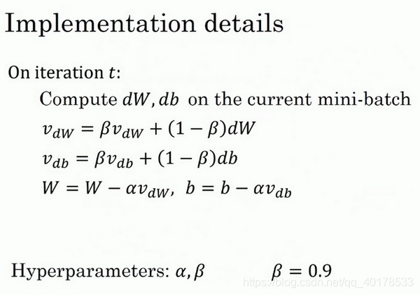
所以你有两个超参数,学习率以及另一个参数,控制着指数加权平均数。另一个参数常为0.9.
RMSprop
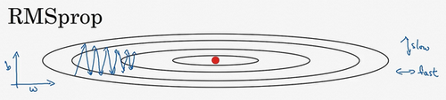
RMSprop的算法,全称是root mean square prop算法,它也可以加速梯度下降,我们来看看它是如何运作的。
回忆一下我们之前的例子,如果你执行梯度下降,虽然横轴方向正在推进,但纵轴方向会有大幅度摆动所以,你想减缓方向b的学习,即纵轴方向,同时加快,至少不是减缓横轴方向的学习,RMSprop算法可以实现这一点。

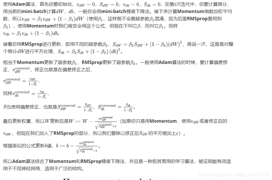
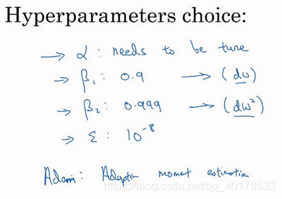
Adam 优化算法(Adam optimization algorithm)
Adam优化算法基本上就是将Momentum和RMSprop结合在一起,那么来看看如何使用Adam算法。
参数选择:
代码
import numpy as np

"""
This file implements various first-order update rules that are commonly used
for training neural networks. Each update rule accepts current weights and the
gradient of the loss with respect to those weights and produces the next set of
weights. Each update rule has the same interface:

def update(w, dw, config=None):

Inputs:
  - w: A numpy array giving the current weights.
  - dw: A numpy array of the same shape as w giving the gradient of the
    loss with respect to w.
  - config: A dictionary containing hyperparameter values such as learning
    rate, momentum, etc. If the update rule requires caching values over many
    iterations, then config will also hold these cached values.

Returns:
  - next_w: The next point after the update.
  - config: The config dictionary to be passed to the next iteration of the
    update rule.

NOTE: For most update rules, the default learning rate will probably not
perform well; however the default values of the other hyperparameters should
work well for a variety of different problems.

For efficiency, update rules may perform in-place updates, mutating w and
setting next_w equal to w.
"""


def sgd(w, dw, config=None):
    """
    Performs vanilla stochastic gradient descent.

    config format:
    - learning_rate: Scalar learning rate.
    """
    if config is None: config = {}
    config.setdefault('learning_rate', 1e-2)

    w -= config['learning_rate'] * dw
    return w, config


def sgd_momentum(w, dw, config=None):
    """
    Performs stochastic gradient descent with momentum.

    config format:
    - learning_rate: Scalar learning rate.
    - momentum: Scalar between 0 and 1 giving the momentum value.
      Setting momentum = 0 reduces to sgd.
    - velocity: A numpy array of the same shape as w and dw used to store a
      moving average of the gradients.
    """
    if config is None: config = {}
    config.setdefault('learning_rate', 1e-2)
    config.setdefault('momentum', 0.9)
    v = config.get('velocity', np.zeros_like(w))

    next_w = None
    ###########################################################################
    # TODO: Implement the momentum update formula. Store the updated value in #
    # the next_w variable. You should also use and update the velocity v.     #
    ###########################################################################
    # *****START OF YOUR CODE (DO NOT DELETE/MODIFY THIS LINE)*****

    v = config['momentum']*v - config['learning_rate']*dw
    next_w = w + v

    # *****END OF YOUR CODE (DO NOT DELETE/MODIFY THIS LINE)*****
    ###########################################################################
    #                             END OF YOUR CODE                            #
    ###########################################################################
    config['velocity'] = v

    return next_w, config


def rmsprop(w, dw, config=None):
    """
    Uses the RMSProp update rule, which uses a moving average of squared
    gradient values to set adaptive per-parameter learning rates.

    config format:
    - learning_rate: Scalar learning rate.
    - decay_rate: Scalar between 0 and 1 giving the decay rate for the squared
      gradient cache.
    - epsilon: Small scalar used for smoothing to avoid dividing by zero.
    - cache: Moving average of second moments of gradients.
    """
    if config is None: config = {}
    config.setdefault('learning_rate', 1e-2)
    config.setdefault('decay_rate', 0.99)
    config.setdefault('epsilon', 1e-8)
    config.setdefault('cache', np.zeros_like(w))

    next_w = None
    ###########################################################################
    # TODO: Implement the RMSprop update formula, storing the next value of w #
    # in the next_w variable. Don't forget to update cache value stored in    #
    # config['cache'].                                                        #
    ###########################################################################
    # *****START OF YOUR CODE (DO NOT DELETE/MODIFY THIS LINE)*****

    cache = config['decay_rate']*config['cache'] + (1-config['decay_rate'])*dw*dw
    config['cache'] = cache
    next_w = w - config['learning_rate']*dw/(np.sqrt(cache)+config['epsilon'])

    # *****END OF YOUR CODE (DO NOT DELETE/MODIFY THIS LINE)*****
    ###########################################################################
    #                             END OF YOUR CODE                            #
    ###########################################################################

    return next_w, config


def adam(w, dw, config=None):
    """
    Uses the Adam update rule, which incorporates moving averages of both the
    gradient and its square and a bias correction term.

    config format:
    - learning_rate: Scalar learning rate.
    - beta1: Decay rate for moving average of first moment of gradient.
    - beta2: Decay rate for moving average of second moment of gradient.
    - epsilon: Small scalar used for smoothing to avoid dividing by zero.
    - m: Moving average of gradient.
    - v: Moving average of squared gradient.
    - t: Iteration number.
    """
    if config is None: config = {}
    config.setdefault('learning_rate', 1e-3)
    config.setdefault('beta1', 0.9)
    config.setdefault('beta2', 0.999)
    config.setdefault('epsilon', 1e-8)
    config.setdefault('m', np.zeros_like(w))
    config.setdefault('v', np.zeros_like(w))
    config.setdefault('t', 0)

    next_w = None
    ###########################################################################
    # TODO: Implement the Adam update formula, storing the next value of w in #
    # the next_w variable. Don't forget to update the m, v, and t variables   #
    # stored in config.                                                       #
    #                                                                         #
    # NOTE: In order to match the reference output, please modify t _before_  #
    # using it in any calculations.                                           #
    ###########################################################################
    # *****START OF YOUR CODE (DO NOT DELETE/MODIFY THIS LINE)*****

    m = config['m']*config['beta1'] + dw*(1-config['beta1'])
    v = config['v']*config['beta2'] + dw*dw*(1-config['beta2'])
    config['m'] = m
    config['v'] = v
    t = config['t'] + 1
    mt = m/(1 - config['beta1']**t)
    vt = v/(1 - config['beta2']**t)
    config['t'] = t
    next_w = w - config['learning_rate']*mt/(np.sqrt(vt)+config['epsilon'])

    # *****END OF YOUR CODE (DO NOT DELETE/MODIFY THIS LINE)*****
    ###########################################################################
    #                             END OF YOUR CODE                            #
    ###########################################################################

    return next_w, config
作业代码
import time
import numpy as np
import matplotlib.pyplot as plt
from cs231n.classifiers.fc_net import *
from cs231n.data_utils import get_CIFAR10_data
from cs231n.gradient_check import eval_numerical_gradient, eval_numerical_gradient_array
from cs231n.solver import Solver

%matplotlib inline
plt.rcParams['figure.figsize'] = (10.0, 8.0) # set default size of plots
plt.rcParams['image.interpolation'] = 'nearest'
plt.rcParams['image.cmap'] = 'gray'

%load_ext autoreload
%autoreload 2

def rel_error(x, y):
    """ returns relative error """
    return np.max(np.abs(x - y) / (np.maximum(1e-8, np.abs(x) + np.abs(y))))

def print_mean_std(x,axis=0):
    print('  means: ', x.mean(axis=axis))
    print('  stds:  ', x.std(axis=axis))
    print()
# 加载数据集
data = get_CIFAR10_data()
for k, v in data.items():
  print('%s: ' % k, v.shape)
# 检查归一化前后的代码
# Simulate the forward pass for a two-layer network
np.random.seed(231)
N, D1, D2, D3 = 200, 50, 60, 3
X = np.random.randn(N, D1)
W1 = np.random.randn(D1, D2)
W2 = np.random.randn(D2, D3)
a = np.maximum(0, X.dot(W1)).dot(W2)

print('Before batch normalization:')
print_mean_std(a,axis=0)

gamma = np.ones((D3,))
beta = np.zeros((D3,))
# Means should be close to zero and stds close to one
print('After batch normalization (gamma=1, beta=0)')
a_norm, _ = batchnorm_forward(a, gamma, beta, {'mode': 'train'})
print_mean_std(a_norm,axis=0)

gamma = np.asarray([1.0, 2.0, 3.0])
beta = np.asarray([11.0, 12.0, 13.0])
# Now means should be close to beta and stds close to gamma
print('After batch normalization (gamma=', gamma, ', beta=', beta, ')')
a_norm, _ = batchnorm_forward(a, gamma, beta, {'mode': 'train'})
print_mean_std(a_norm,axis=0)
np.random.seed(231)
N, D1, D2, D3 = 200, 50, 60, 3
W1 = np.random.randn(D1, D2)
W2 = np.random.randn(D2, D3)

bn_param = {'mode': 'train'}
gamma = np.ones(D3)
beta = np.zeros(D3)

for t in range(50):
  X = np.random.randn(N, D1)
  a = np.maximum(0, X.dot(W1)).dot(W2)
  batchnorm_forward(a, gamma, beta, bn_param)

bn_param['mode'] = 'test'
X = np.random.randn(N, D1)
a = np.maximum(0, X.dot(W1)).dot(W2)
a_norm, _ = batchnorm_forward(a, gamma, beta, bn_param)

# Means should be close to zero and stds close to one, but will be
# noisier than training-time forward passes.
print('After batch normalization (test-time):')
print_mean_std(a_norm,axis=0)
# 检查 batchnorm 的梯度
np.random.seed(231)
N, D = 4, 5
x = 5 * np.random.randn(N, D) + 12
gamma = np.random.randn(D)
beta = np.random.randn(D)
dout = np.random.randn(N, D)

bn_param = {'mode': 'train'}
fx = lambda x: batchnorm_forward(x, gamma, beta, bn_param)[0]
fg = lambda a: batchnorm_forward(x, a, beta, bn_param)[0]
fb = lambda b: batchnorm_forward(x, gamma, b, bn_param)[0]

dx_num = eval_numerical_gradient_array(fx, x, dout)
da_num = eval_numerical_gradient_array(fg, gamma.copy(), dout)
db_num = eval_numerical_gradient_array(fb, beta.copy(), dout)

_, cache = batchnorm_forward(x, gamma, beta, bn_param)
dx, dgamma, dbeta = batchnorm_backward(dout, cache)
#You should expect to see relative errors between 1e-13 and 1e-8
print('dx error: ', rel_error(dx_num, dx))
print('dgamma error: ', rel_error(da_num, dgamma))
print('dbeta error: ', rel_error(db_num, dbeta))
np.random.seed(231)
N, D = 100, 500
x = 5 * np.random.randn(N, D) + 12
gamma = np.random.randn(D)
beta = np.random.randn(D)
dout = np.random.randn(N, D)

bn_param = {'mode': 'train'}
out, cache = batchnorm_forward(x, gamma, beta, bn_param)

t1 = time.time()
dx1, dgamma1, dbeta1 = batchnorm_backward(dout, cache)
t2 = time.time()
dx2, dgamma2, dbeta2 = batchnorm_backward_alt(dout, cache)
t3 = time.time()

print('dx difference: ', rel_error(dx1, dx2))
print('dgamma difference: ', rel_error(dgamma1, dgamma2))
print('dbeta difference: ', rel_error(dbeta1, dbeta2))
print('speedup: %.2fx' % ((t2 - t1) / (t3 - t2)))
np.random.seed(231)
N, D, H1, H2, C = 2, 15, 20, 30, 10
X = np.random.randn(N, D)
y = np.random.randint(C, size=(N,))

# You should expect losses between 1e-4~1e-10 for W,
# losses between 1e-08~1e-10 for b,
# and losses between 1e-08~1e-09 for beta and gammas.
for reg in [0, 3.14]:
  print('Running check with reg = ', reg)
  model = FullyConnectedNet([H1, H2], input_dim=D, num_classes=C,
                            reg=reg, weight_scale=5e-2, dtype=np.float64,
                            normalization='batchnorm')

  loss, grads = model.loss(X, y)
  print('Initial loss: ', loss)

  for name in sorted(grads):
    f = lambda _: model.loss(X, y)[0]
    grad_num = eval_numerical_gradient(f, model.params[name], verbose=False, h=1e-5)
    print('%s relative error: %.2e' % (name, rel_error(grad_num, grads[name])))
  if reg == 0: print()
np.random.seed(231)
# T在深度神经网络中训练batchNorm
hidden_dims = [100, 100, 100, 100, 100]

num_train = 1000
small_data = {
  'X_train': data['X_train'][:num_train],
  'y_train': data['y_train'][:num_train],
  'X_val': data['X_val'],
  'y_val': data['y_val'],
}

weight_scale = 2e-2
bn_model = FullyConnectedNet(hidden_dims, weight_scale=weight_scale, normalization='batchnorm')
model = FullyConnectedNet(hidden_dims, weight_scale=weight_scale, normalization=None)

print('Solver with batch norm:')
bn_solver = Solver(bn_model, small_data,
                num_epochs=10, batch_size=50,
                update_rule='adam',
                optim_config={
                  'learning_rate': 1e-3,
                },
                verbose=True,print_every=20)
bn_solver.train()

print('\nSolver without batch norm:')
solver = Solver(model, small_data,
                num_epochs=10, batch_size=50,
                update_rule='adam',
                optim_config={
                  'learning_rate': 1e-3,
                },
                verbose=True, print_every=20)
solver.train()
def plot_training_history(title, label, baseline, bn_solvers, plot_fn, bl_marker='.', bn_marker='.', labels=None):
    """utility function for plotting training history"""
    plt.title(title)
    plt.xlabel(label)
    bn_plots = [plot_fn(bn_solver) for bn_solver in bn_solvers]
    bl_plot = plot_fn(baseline)
    num_bn = len(bn_plots)
    for i in range(num_bn):
        label='with_norm'
        if labels is not None:
            label += str(labels[i])
        plt.plot(bn_plots[i], bn_marker, label=label)
    label='baseline'
    if labels is not None:
        label += str(labels[0])
    plt.plot(bl_plot, bl_marker, label=label)
    plt.legend(loc='lower center', ncol=num_bn+1)


plt.subplot(3, 1, 1)
plot_training_history('Training loss','Iteration', solver, [bn_solver], \
                      lambda x: x.loss_history, bl_marker='o', bn_marker='o')
plt.subplot(3, 1, 2)
plot_training_history('Training accuracy','Epoch', solver, [bn_solver], \
                      lambda x: x.train_acc_history, bl_marker='-o', bn_marker='-o')
plt.subplot(3, 1, 3)
plot_training_history('Validation accuracy','Epoch', solver, [bn_solver], \
                      lambda x: x.val_acc_history, bl_marker='-o', bn_marker='-o')

plt.gcf().set_size_inches(15, 15)
plt.show()
# 研究批次归一化和权重初始化的相互作
np.random.seed(231)
# Try training a very deep net with batchnorm
hidden_dims = [50, 50, 50, 50, 50, 50, 50]
num_train = 1000
small_data = {
  'X_train': data['X_train'][:num_train],
  'y_train': data['y_train'][:num_train],
  'X_val': data['X_val'],
  'y_val': data['y_val'],
}

bn_solvers_ws = {}
solvers_ws = {}
weight_scales = np.logspace(-4, 0, num=20)
for i, weight_scale in enumerate(weight_scales):
  print('Running weight scale %d / %d' % (i + 1, len(weight_scales)))
  bn_model = FullyConnectedNet(hidden_dims, weight_scale=weight_scale, normalization='batchnorm')
  model = FullyConnectedNet(hidden_dims, weight_scale=weight_scale, normalization=None)

  bn_solver = Solver(bn_model, small_data,
                  num_epochs=10, batch_size=50,
                  update_rule='adam',
                  optim_config={
                    'learning_rate': 1e-3,
                  },
                  verbose=False, print_every=200)
  bn_solver.train()
  bn_solvers_ws[weight_scale] = bn_solver

  solver = Solver(model, small_data,
                  num_epochs=10, batch_size=50,
                  update_rule='adam',
                  optim_config={
                    'learning_rate': 1e-3,
                  },
                  verbose=False, print_every=200)
  solver.train()
  solvers_ws[weight_scale] = solver
# Plot results of weight scale experiment
best_train_accs, bn_best_train_accs = [], []
best_val_accs, bn_best_val_accs = [], []
final_train_loss, bn_final_train_loss = [], []

for ws in weight_scales:
  best_train_accs.append(max(solvers_ws[ws].train_acc_history))
  bn_best_train_accs.append(max(bn_solvers_ws[ws].train_acc_history))

  best_val_accs.append(max(solvers_ws[ws].val_acc_history))
  bn_best_val_accs.append(max(bn_solvers_ws[ws].val_acc_history))

  final_train_loss.append(np.mean(solvers_ws[ws].loss_history[-100:]))
  bn_final_train_loss.append(np.mean(bn_solvers_ws[ws].loss_history[-100:]))

plt.subplot(3, 1, 1)
plt.title('Best val accuracy vs weight initialization scale')
plt.xlabel('Weight initialization scale')
plt.ylabel('Best val accuracy')
plt.semilogx(weight_scales, best_val_accs, '-o', label='baseline')
plt.semilogx(weight_scales, bn_best_val_accs, '-o', label='batchnorm')
plt.legend(ncol=2, loc='lower right')

plt.subplot(3, 1, 2)
plt.title('Best train accuracy vs weight initialization scale')
plt.xlabel('Weight initialization scale')
plt.ylabel('Best training accuracy')
plt.semilogx(weight_scales, best_train_accs, '-o', label='baseline')
plt.semilogx(weight_scales, bn_best_train_accs, '-o', label='batchnorm')
plt.legend()

plt.subplot(3, 1, 3)
plt.title('Final training loss vs weight initialization scale')
plt.xlabel('Weight initialization scale')
plt.ylabel('Final training loss')
plt.semilogx(weight_scales, final_train_loss, '-o', label='baseline')
plt.semilogx(weight_scales, bn_final_train_loss, '-o', label='batchnorm')
plt.legend()
plt.gca().set_ylim(1.0, 3.5)

plt.gcf().set_size_inches(15, 15)
plt.show()
# 现在,我们将运行一个小实验来研究批处理规范化和批处理大小的相互作用。
def run_batchsize_experiments(normalization_mode):
    np.random.seed(231)
    # Try training a very deep net with batchnorm
    hidden_dims = [100, 100, 100, 100, 100]
    num_train = 1000
    small_data = {
      'X_train': data['X_train'][:num_train],
      'y_train': data['y_train'][:num_train],
      'X_val': data['X_val'],
      'y_val': data['y_val'],
    }
    n_epochs=10
    weight_scale = 2e-2
    batch_sizes = [5,10,50]
    lr = 10**(-3.5)
    solver_bsize = batch_sizes[0]

    print('No normalization: batch size = ',solver_bsize)
    model = FullyConnectedNet(hidden_dims, weight_scale=weight_scale, normalization=None)
    solver = Solver(model, small_data,
                    num_epochs=n_epochs, batch_size=solver_bsize,
                    update_rule='adam',
                    optim_config={
                      'learning_rate': lr,
                    },
                    verbose=False)
    solver.train()

    bn_solvers = []
    for i in range(len(batch_sizes)):
        b_size=batch_sizes[i]
        print('Normalization: batch size = ',b_size)
        bn_model = FullyConnectedNet(hidden_dims, weight_scale=weight_scale, normalization=normalization_mode)
        bn_solver = Solver(bn_model, small_data,
                        num_epochs=n_epochs, batch_size=b_size,
                        update_rule='adam',
                        optim_config={
                          'learning_rate': lr,
                        },
                        verbose=False)
        bn_solver.train()
        bn_solvers.append(bn_solver)

    return bn_solvers, solver, batch_sizes

batch_sizes = [5,10,50]
bn_solvers_bsize, solver_bsize, batch_sizes = run_batchsize_experiments('batchnorm')
# 绘制图像
plt.subplot(2, 1, 1)
plot_training_history('Training accuracy (Batch Normalization)','Epoch', solver_bsize, bn_solvers_bsize, \
                      lambda x: x.train_acc_history, bl_marker='-^', bn_marker='-o', labels=batch_sizes)
plt.subplot(2, 1, 2)
plot_training_history('Validation accuracy (Batch Normalization)','Epoch', solver_bsize, bn_solvers_bsize, \
                      lambda x: x.val_acc_history, bl_marker='-^', bn_marker='-o', labels=batch_sizes)

plt.gcf().set_size_inches(15, 10)
plt.show()
# 批处理规范化已被证明可以有效地使网络更容易训练,
# 但是对批处理大小的依赖性使其在复杂网络中的用处不大,
# 而复杂网络由于硬件限制而限制了输入批处理大小。

# 为了缓解这个问题,已经提出了几种批处理标准化的替代方法。
# 一种这样的技术是层归一化[2]。 我们没有对批处理进行标准化,
# 而是对功能进行了标准化。换句话说,当使用“层归一化”时,
# 将基于该特征向量内所有项的总和对与单个数据点相对应的每个特征向量进行归一化。
np.random.seed(231)
N, D1, D2, D3 =4, 50, 60, 3
X = np.random.randn(N, D1)
W1 = np.random.randn(D1, D2)
W2 = np.random.randn(D2, D3)
a = np.maximum(0, X.dot(W1)).dot(W2)

print('Before layer normalization:')
print_mean_std(a,axis=1)

gamma = np.ones(D3)
beta = np.zeros(D3)
# Means should be close to zero and stds close to one
print('After layer normalization (gamma=1, beta=0)')
a_norm, _ = layernorm_forward(a, gamma, beta, {'mode': 'train'})
print_mean_std(a_norm,axis=1)

gamma = np.asarray([3.0,3.0,3.0])
beta = np.asarray([5.0,5.0,5.0])
# Now means should be close to beta and stds close to gamma
print('After layer normalization (gamma=', gamma, ', beta=', beta, ')')
a_norm, _ = layernorm_forward(a, gamma, beta, {'mode': 'train'})
print_mean_std(a_norm,axis=1)

# Gradient check batchnorm backward pass
np.random.seed(231)
N, D = 4, 5
x = 5 * np.random.randn(N, D) + 12
gamma = np.random.randn(D)
beta = np.random.randn(D)
dout = np.random.randn(N, D)

ln_param = {}
fx = lambda x: layernorm_forward(x, gamma, beta, ln_param)[0]
fg = lambda a: layernorm_forward(x, a, beta, ln_param)[0]
fb = lambda b: layernorm_forward(x, gamma, b, ln_param)[0]

dx_num = eval_numerical_gradient_array(fx, x, dout)
da_num = eval_numerical_gradient_array(fg, gamma.copy(), dout)
db_num = eval_numerical_gradient_array(fb, beta.copy(), dout)

_, cache = layernorm_forward(x, gamma, beta, ln_param)
dx, dgamma, dbeta = layernorm_backward(dout, cache)

#You should expect to see relative errors between 1e-12 and 1e-8
print('dx error: ', rel_error(dx_num, dx))
print('dgamma error: ', rel_error(da_num, dgamma))
print('dbeta error: ', rel_error(db_num, dbeta))
ln_solvers_bsize, solver_bsize, batch_sizes = run_batchsize_experiments('layernorm')

plt.subplot(2, 1, 1)
plot_training_history('Training accuracy (Layer Normalization)','Epoch', solver_bsize, ln_solvers_bsize, \
                      lambda x: x.train_acc_history, bl_marker='-^', bn_marker='-o', labels=batch_sizes)
plt.subplot(2, 1, 2)
plot_training_history('Validation accuracy (Layer Normalization)','Epoch', solver_bsize, ln_solvers_bsize, \
                      lambda x: x.val_acc_history, bl_marker='-^', bn_marker='-o', labels=batch_sizes)

plt.gcf().set_size_inches(15, 10)
plt.show()