Initialization
获取数据,其中init_utils的文件在文章最后附录中
主要内容:初始化权重的比较
输入:
import numpy as np
import matplotlib.pyplot as plt
import sklearn
import sklearn.datasets
from init_utils import sigmoid, relu, compute_loss, forward_propagation, backward_propagation
from init_utils import update_parameters, predict, load_dataset, plot_decision_boundary, predict_dec

plt.rcParams['figure.figsize'] = (7.0, 4.0) # set default size of plots
plt.rcParams['image.interpolation'] = 'nearest'
plt.rcParams['image.cmap'] = 'gray'

# load image dataset: blue/red dots in circles
train_X, train_Y, test_X, test_Y = load_dataset()
输出:

1 - Neural Network model
You will use a 3-layer neural network (already implemented for you). Here are the initialization methods you will experiment with:
- Zeros initialization -- setting
initialization = "zeros"in the input argument. - Random initialization -- setting
initialization = "random"in the input argument. This initializes the weights to large random values. - He initialization -- setting
initialization = "he"in the input argument. This initializes the weights to random values scaled according to a paper by He et al., 2015.
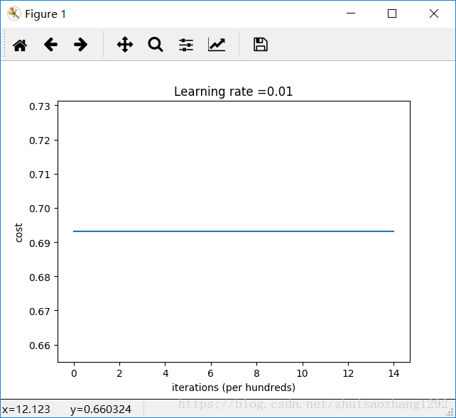
2 - Zero initialization
There are two types of parameters to initialize in a neural network:
- the weight matrices (W[1],W[2],W[3],...,W[L−1],W[L])(W[1],W[2],W[3],...,W[L−1],W[L])
- the bias vectors (b[1],b[2],b[3],...,b[L−1],b[L])(b[1],b[2],b[3],...,b[L−1],b[L])
Exercise: Implement the following function to initialize all parameters to zeros. You’ll see later that this does not work well since it fails to “break symmetry”, but lets try it anyway and see what happens. Use np.zeros((..,..)) with the correct shapes.
输入:
def model(X, Y, learning_rate = 0.01, num_iterations = 15000, print_cost = True, initialization = "he"):
    """
    Implements a three-layer neural network: LINEAR->RELU->LINEAR->RELU->LINEAR->SIGMOID.

    Arguments:
    X -- input data, of shape (2, number of examples)
    Y -- true "label" vector (containing 0 for red dots; 1 for blue dots), of shape (1, number of examples)
    learning_rate -- learning rate for gradient descent
    num_iterations -- number of iterations to run gradient descent
    print_cost -- if True, print the cost every 1000 iterations
    initialization -- flag to choose which initialization to use ("zeros","random" or "he")

    Returns:
    parameters -- parameters learnt by the model
    """

    grads = {}
    costs = [] # to keep track of the loss
    m = X.shape[1] # number of examples
    layers_dims = [X.shape[0], 10, 5, 1]

    # Initialize parameters dictionary.
    if initialization == "zeros":
        parameters = initialize_parameters_zeros(layers_dims)
    elif initialization == "random":
        parameters = initialize_parameters_random(layers_dims)
    elif initialization == "he":
        parameters = initialize_parameters_he(layers_dims)

    # Loop (gradient descent)

    for i in range(0, num_iterations):

        # Forward propagation: LINEAR -> RELU -> LINEAR -> RELU -> LINEAR -> SIGMOID.
        a3, cache = forward_propagation(X, parameters)

        # Loss
        cost = compute_loss(a3, Y)

        # Backward propagation.
        grads = backward_propagation(X, Y, cache)

        # Update parameters.
        parameters = update_parameters(parameters, grads, learning_rate)

        # Print the loss every 1000 iterations
        if print_cost and i % 1000 == 0:
            print("Cost after iteration {}: {}".format(i, cost))
            costs.append(cost)

    # plot the loss
    plt.plot(costs)
    plt.ylabel('cost')
    plt.xlabel('iterations (per hundreds)')
    plt.title("Learning rate =" + str(learning_rate))
    plt.show()

    return parameters

def initialize_parameters_zeros(layers_dims):
    """
    Arguments:
    layer_dims -- python array (list) containing the size of each layer.

    Returns:
    parameters -- python dictionary containing your parameters "W1", "b1", ..., "WL", "bL":
                    W1 -- weight matrix of shape (layers_dims[1], layers_dims[0])
                    b1 -- bias vector of shape (layers_dims[1], 1)
                    ...
                    WL -- weight matrix of shape (layers_dims[L], layers_dims[L-1])
                    bL -- bias vector of shape (layers_dims[L], 1)
    """

    parameters = {}
    L = len(layers_dims)            # number of layers in the network

    for l in range(1, L):
        ### START CODE HERE ### (≈ 2 lines of code)
        parameters['W' + str(l)] = np.zeros((layers_dims[l],layers_dims[l-1]))
        parameters['b' + str(l)] = np.zeros((layers_dims[l],1))
        ### END CODE HERE ###
    return parameters
输出:
Cost after iteration 0: 0.6931471805599453
Cost after iteration 1000: 0.6931471805599453
Cost after iteration 2000: 0.6931471805599453
Cost after iteration 3000: 0.6931471805599453
Cost after iteration 4000: 0.6931471805599453
Cost after iteration 5000: 0.6931471805599453
Cost after iteration 6000: 0.6931471805599453
Cost after iteration 7000: 0.6931471805599453
Cost after iteration 8000: 0.6931471805599453
Cost after iteration 9000: 0.6931471805599453
Cost after iteration 10000: 0.6931471805599455
Cost after iteration 11000: 0.6931471805599453
Cost after iteration 12000: 0.6931471805599453
Cost after iteration 13000: 0.6931471805599453
Cost after iteration 14000: 0.6931471805599453
On the train set:
Accuracy: 0.5
On the test set:
Accuracy: 0.5
print ("predictions_train = " + str(predictions_train))
print ("predictions_test = " + str(predictions_test))
predictions_train = [[0 0 0 0 0 0 0 0 0 0 0 0 0 0 0 0 0 0 0 0 0 0 0 0 0 0 0 0 0 0 0 0 0 0 0 0 0
0 0 0 0 0 0 0 0 0 0 0 0 0 0 0 0 0 0 0 0 0 0 0 0 0 0 0 0 0 0 0 0 0 0 0 0 0
0 0 0 0 0 0 0 0 0 0 0 0 0 0 0 0 0 0 0 0 0 0 0 0 0 0 0 0 0 0 0 0 0 0 0 0 0
0 0 0 0 0 0 0 0 0 0 0 0 0 0 0 0 0 0 0 0 0 0 0 0 0 0 0 0 0 0 0 0 0 0 0 0 0
0 0 0 0 0 0 0 0 0 0 0 0 0 0 0 0 0 0 0 0 0 0 0 0 0 0 0 0 0 0 0 0 0 0 0 0 0
0 0 0 0 0 0 0 0 0 0 0 0 0 0 0 0 0 0 0 0 0 0 0 0 0 0 0 0 0 0 0 0 0 0 0 0 0
0 0 0 0 0 0 0 0 0 0 0 0 0 0 0 0 0 0 0 0 0 0 0 0 0 0 0 0 0 0 0 0 0 0 0 0 0
0 0 0 0 0 0 0 0 0 0 0 0 0 0 0 0 0 0 0 0 0 0 0 0 0 0 0 0 0 0 0 0 0 0 0 0 0
0 0 0 0]]
predictions_test = [[0 0 0 0 0 0 0 0 0 0 0 0 0 0 0 0 0 0 0 0 0 0 0 0 0 0 0 0 0 0 0 0 0 0 0 0 0
0 0 0 0 0 0 0 0 0 0 0 0 0 0 0 0 0 0 0 0 0 0 0 0 0 0 0 0 0 0 0 0 0 0 0 0 0
0 0 0 0 0 0 0 0 0 0 0 0 0 0 0 0 0 0 0 0 0 0 0 0 0 0]]
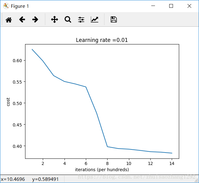
3 - Random initialization
To break symmetry, lets intialize the weights randomly. Following random initialization, each neuron can then proceed to learn a different function of its inputs. In this exercise, you will see what happens if the weights are intialized randomly, but to very large values.
parameters = initialize_parameters_random([3, 2, 1])
print("W1 = " + str(parameters["W1"]))
print("b1 = " + str(parameters["b1"]))
print("W2 = " + str(parameters["W2"]))
print("b2 = " + str(parameters["b2"]))
输出:
W1 = [[ 17.88628473   4.36509851   0.96497468]
 [-18.63492703  -2.77388203  -3.54758979]]
b1 = [[ 0.]
 [ 0.]]
W2 = [[-0.82741481 -6.27000677]]
b2 = [[ 0.]]
输入:
parameters = model(train_X, train_Y, initialization = "random")
print ("On the train set:")
predictions_train = predict(train_X, train_Y, parameters)
print ("On the test set:")
predictions_test = predict(test_X, test_Y, parameters)
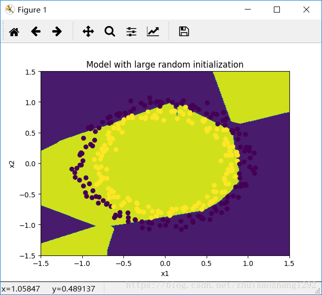
plt.title("Model with large random initialization")
axes = plt.gca()
axes.set_xlim([-1.5,1.5])
axes.set_ylim([-1.5,1.5])
plot_decision_boundary(lambda x: predict_dec(parameters, x.T), train_X, np.squeeze(train_Y))输出:
If you see “inf” as the cost after the iteration 0, this is because of numerical roundoff; a more numerically sophisticated implementation would fix this. But this isn’t worth worrying about for our purposes
D:\F\eclipse-workspace\deep_learning\src\init_utils.py:157: RuntimeWarning: divide by zero encountered in log
  logprobs = np.multiply(-np.log(a3),Y) + np.multiply(-np.log(1 - a3), 1 - Y)
Cost after iteration 0: inf
D:\F\eclipse-workspace\deep_learning\src\init_utils.py:157: RuntimeWarning: invalid value encountered in multiply
  logprobs = np.multiply(-np.log(a3),Y) + np.multiply(-np.log(1 - a3), 1 - Y)
Cost after iteration 1000: 0.6250982793959966
Cost after iteration 2000: 0.5981216596703697
Cost after iteration 3000: 0.5638417572298645
Cost after iteration 4000: 0.5501703049199763
Cost after iteration 5000: 0.5444632909664456
Cost after iteration 6000: 0.5374513807000807
Cost after iteration 7000: 0.4764042074074983
Cost after iteration 8000: 0.39781492295092263
Cost after iteration 9000: 0.3934764028765484
Cost after iteration 10000: 0.3920295461882659
Cost after iteration 11000: 0.38924598135108
Cost after iteration 12000: 0.3861547485712325
Cost after iteration 13000: 0.384984728909703
Cost after iteration 14000: 0.3827828308349524
On the train set:
Accuracy: 0.83
On the test set:
Accuracy: 0.86
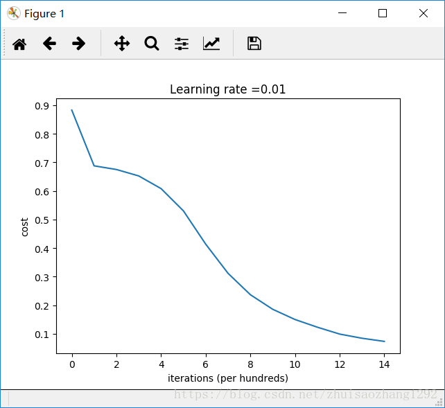
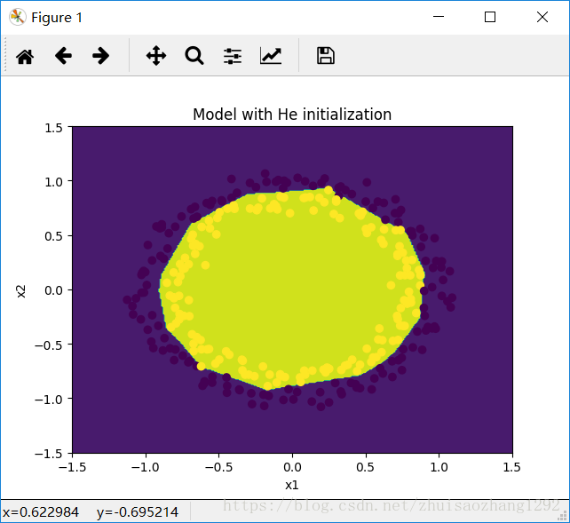
4 - He initialization
Finally, try “He Initialization”; this is named for the first author of He et al., 2015. (If you have heard of “Xavier initialization”, this is similar except Xavier initialization uses a scaling factor for the weights W[l]W[l] of sqrt(1./layers_dims[l-1]) where He initialization would use sqrt(2./layers_dims[l-1]).)
Exercise: Implement the following function to initialize your parameters with He initialization.
Hint: This function is similar to the previous initialize_parameters_random(...). The only difference is that instead of multiplying np.random.randn(..,..) by 10, you will multiply it by 2dimension of the previous layer−−−−−−−−−−−−−−−−−−√2dimension of the previous layer, which is what He initialization recommends for layers with a ReLU activation.
输入:
parameters = model(train_X, train_Y, initialization = "he")
print ("On the train set:")
predictions_train = predict(train_X, train_Y, parameters)
print ("On the test set:")
predictions_test = predict(test_X, test_Y, parameters)

plt.title("Model with He initialization")
axes = plt.gca()
axes.set_xlim([-1.5,1.5])
axes.set_ylim([-1.5,1.5])
plot_decision_boundary(lambda x: predict_dec(parameters, x.T), train_X, np.squeeze(train_Y))
输出:
Cost after iteration 0: 0.8830537463419761
Cost after iteration 1000: 0.6879825919728063
Cost after iteration 2000: 0.6751286264523371
Cost after iteration 3000: 0.6526117768893807
Cost after iteration 4000: 0.6082958970572937
Cost after iteration 5000: 0.5304944491717495
Cost after iteration 6000: 0.4138645817071793
Cost after iteration 7000: 0.3117803464844441
Cost after iteration 8000: 0.23696215330322556
Cost after iteration 9000: 0.18597287209206828
Cost after iteration 10000: 0.15015556280371808
Cost after iteration 11000: 0.12325079292273548
Cost after iteration 12000: 0.09917746546525937
Cost after iteration 13000: 0.08457055954024274
Cost after iteration 14000: 0.07357895962677366
On the train set:
Accuracy: 0.993333333333
On the test set:
Accuracy: 0.96
附录:
init_utils.py
# -*- coding: utf-8 -*-
"""
Created on Sat Apr 21 21:58:39 2018

@author: StephenGai
"""
import numpy as np
import matplotlib.pyplot as plt
import h5py
import sklearn
import sklearn.datasets

def setcolor(x):
    color=[]
    for i in range(x.shape[1]):
        if x[:,i]==1:
            color.append('b')
        else:
            color.append('r')
    return color

def sigmoid(x):
    """
    Compute the sigmoid of x

    Arguments:
    x -- A scalar or numpy array of any size.

    Return:
    s -- sigmoid(x)
    """
    s = 1/(1+np.exp(-x))
    return s

def relu(x):
    """
    Compute the relu of x

    Arguments:
    x -- A scalar or numpy array of any size.

    Return:
    s -- relu(x)
    """
    s = np.maximum(0,x)

    return s

def forward_propagation(X, parameters):
    """
    Implements the forward propagation (and computes the loss) presented in Figure 2.

    Arguments:
    X -- input dataset, of shape (input size, number of examples)
    Y -- true "label" vector (containing 0 if cat, 1 if non-cat)
    parameters -- python dictionary containing your parameters "W1", "b1", "W2", "b2", "W3", "b3":
                    W1 -- weight matrix of shape ()
                    b1 -- bias vector of shape ()
                    W2 -- weight matrix of shape ()
                    b2 -- bias vector of shape ()
                    W3 -- weight matrix of shape ()
                    b3 -- bias vector of shape ()

    Returns:
    loss -- the loss function (vanilla logistic loss)
    """
    # retrieve parameters
    W1 = parameters["W1"]
    b1 = parameters["b1"]
    W2 = parameters["W2"]
    b2 = parameters["b2"]
    W3 = parameters["W3"]
    b3 = parameters["b3"]

    # LINEAR -> RELU -> LINEAR -> RELU -> LINEAR -> SIGMOID
    z1 = np.dot(W1, X)  + b1
    a1 = relu(z1)
    z2 = np.dot(W2, a1) + b2
    a2 = relu(z2)
    z3 = np.dot(W3, a2) + b3
    a3 = sigmoid(z3)

    cache = (z1, a1, W1, b1, z2, a2, W2, b2, z3, a3, W3, b3)

    return a3, cache

def backward_propagation(X, Y, cache):
    """
    Implement the backward propagation presented in figure 2.

    Arguments:
    X -- input dataset, of shape (input size, number of examples)
    Y -- true "label" vector (containing 0 if cat, 1 if non-cat)
    cache -- cache output from forward_propagation()

    Returns:
    gradients -- A dictionary with the gradients with respect to each parameter, activation and pre-activation variables
    """
    m = X.shape[1]
    (z1, a1, W1, b1, z2, a2, W2, b2, z3, a3, W3, b3) = cache

    dz3 = 1./m * (a3 - Y)
    dW3 = np.dot(dz3, a2.T)
    db3 = np.sum(dz3, axis=1, keepdims = True)

    da2 = np.dot(W3.T, dz3)
    dz2 = np.multiply(da2, np.int64(a2 > 0))
    dW2 = np.dot(dz2, a1.T)
    db2 = np.sum(dz2, axis=1, keepdims = True)

    da1 = np.dot(W2.T, dz2)
    dz1 = np.multiply(da1, np.int64(a1 > 0))
    dW1 = np.dot(dz1, X.T)
    db1 = np.sum(dz1, axis=1, keepdims = True)

    gradients = {"dz3": dz3, "dW3": dW3, "db3": db3,
                 "da2": da2, "dz2": dz2, "dW2": dW2, "db2": db2,
                 "da1": da1, "dz1": dz1, "dW1": dW1, "db1": db1}

    return gradients

def update_parameters(parameters, grads, learning_rate):
    """
    Update parameters using gradient descent

    Arguments:
    parameters -- python dictionary containing your parameters
    grads -- python dictionary containing your gradients, output of n_model_backward

    Returns:
    parameters -- python dictionary containing your updated parameters
                  parameters['W' + str(i)] = ...
                  parameters['b' + str(i)] = ...
    """
    L = len(parameters) // 2 # number of layers in the neural networks

    # Update rule for each parameter
    for k in range(L):
        parameters["W" + str(k+1)] = parameters["W" + str(k+1)] - learning_rate * grads["dW" + str(k+1)]
        parameters["b" + str(k+1)] = parameters["b" + str(k+1)] - learning_rate * grads["db" + str(k+1)]

    return parameters

def compute_loss(a3, Y):

    """
    Implement the loss function

    Arguments:
    a3 -- post-activation, output of forward propagation
    Y -- "true" labels vector, same shape as a3

    Returns:
    loss - value of the loss function
    """
    m = Y.shape[1]
    logprobs = np.multiply(-np.log(a3),Y) + np.multiply(-np.log(1 - a3), 1 - Y)
    loss = 1./m * np.nansum(logprobs)

    return loss

def predict(X, y, parameters):
    """
    This function is used to predict the results of a  n-layer neural network.

    Arguments:
    X -- data set of examples you would like to label
    parameters -- parameters of the trained model

    Returns:
    p -- predictions for the given dataset X
    """
    m = X.shape[1]
    p = np.zeros((1,m), dtype = np.int)

    # Forward propagation
    a3, caches = forward_propagation(X, parameters)

    # convert probas to 0/1 predictions
    for i in range(0, a3.shape[1]):
        if a3[0,i] > 0.5:
            p[0,i] = 1
        else:
            p[0,i] = 0

    # print results
    print("Accuracy: "  + str(np.mean((p[0,:] == y[0,:]))))

    return p

# def plot_decision_boundary(model, X, y):
#     # Set min and max values and give it some padding
#     x_min, x_max = X[0, :].min() - 1, X[0, :].max() + 1
#     y_min, y_max = X[1, :].min() - 1, X[1, :].max() + 1
#     h = 0.01
#     # Generate a grid of points with distance h between them
#     xx, yy = np.meshgrid(np.arange(x_min, x_max, h), np.arange(y_min, y_max, h))
#     # Predict the function value for the whole grid
#     Z = model(np.c_[xx.ravel(), yy.ravel()])
#     Z = Z.reshape(xx.shape)
#     # Plot the contour and training examples
#     plt.contourf(xx, yy, Z)
#     plt.ylabel('x2')
#     plt.xlabel('x1')
#     plt.scatter(X[0, :], X[1, :], c=setcolor(y))
#     plt.show()

def plot_decision_boundary(model, X, y):
    # Set min and max values and give it some padding
    x_min, x_max = X[0, :].min() - 1, X[0, :].max() + 1
    y_min, y_max = X[1, :].min() - 1, X[1, :].max() + 1
    h = 0.01
    # Generate a grid of points with distance h between them

    xx, yy = np.meshgrid(np.arange(x_min, x_max, h), np.arange(y_min, y_max, h))
    # Predict the function value for the whole grid
    Z = model(np.c_[xx.ravel(), yy.ravel()])
    Z = Z.reshape(xx.shape)

    # Plot the contour and training examples
    plt.contourf(xx, yy, Z)
    plt.ylabel('x2')
    plt.xlabel('x1')
    plt.scatter(X[0, :], X[1, :], c=y)
    plt.show()

def predict_dec(parameters, X):
    """
    Used for plotting decision boundary.

    Arguments:
    parameters -- python dictionary containing your parameters
    X -- input data of size (m, K)

    Returns
    predictions -- vector of predictions of our model (red: 0 / blue: 1)
    """
    # Predict using forward propagation and a classification threshold of 0.5
    a3, cache = forward_propagation(X, parameters)
    predictions = (a3>0.5)
    return predictions

def load_dataset():
    np.random.seed(1)
    train_X, train_Y = sklearn.datasets.make_circles(n_samples=300, noise=.05)
    np.random.seed(2)
    test_X, test_Y = sklearn.datasets.make_circles(n_samples=100, noise=.05)

    train_X = train_X.T
    train_Y = train_Y.reshape((1, train_Y.shape[0]))
    test_X = test_X.T
    test_Y = test_Y.reshape((1, test_Y.shape[0]))

    # Visualize the data
    plt.scatter(train_X[0,:], train_X[1,:], c=setcolor(train_Y), s=40)
    plt.show()

    return train_X, train_Y, test_X, test_Y

def load_cat_dataset():
    train_dataset = h5py.File('datasets/train_catvnoncat.h5', "r")
    train_set_x_orig = np.array(train_dataset["train_set_x"][:]) # your train set features
    train_set_y_orig = np.array(train_dataset["train_set_y"][:]) # your train set labels

    test_dataset = h5py.File('datasets/test_catvnoncat.h5', "r")
    test_set_x_orig = np.array(test_dataset["test_set_x"][:]) # your test set features
    test_set_y_orig = np.array(test_dataset["test_set_y"][:]) # your test set labels

    classes = np.array(test_dataset["list_classes"][:]) # the list of classes

    train_set_y = train_set_y_orig.reshape((1, train_set_y_orig.shape[0]))
    test_set_y = test_set_y_orig.reshape((1, test_set_y_orig.shape[0]))

    train_set_x_orig = train_set_x_orig.reshape(train_set_x_orig.shape[0], -1).T
    test_set_x_orig = test_set_x_orig.reshape(test_set_x_orig.shape[0], -1).T

    train_set_x = train_set_x_orig/255
    test_set_x = test_set_x_orig/255

    return train_set_x, train_set_y, test_set_x, test_set_y, classes