Gradient Checking
Welcome to the final assignment for this week! In this assignment you will learn to implement and use gradient checking.
You are part of a team working to make mobile payments available globally, and are asked to build a deep learning model to detect fraud--whenever someone makes a payment, you want to see if the payment might be fraudulent, such as if the user's account has been taken over by a hacker.
But backpropagation is quite challenging to implement, and sometimes has bugs. Because this is a mission-critical application, your company's CEO wants to be really certain that your implementation of backpropagation is correct. Your CEO says, "Give me a proof that your backpropagation is actually working!" To give this reassurance, you are going to use "gradient checking".
Let's do it!
# Packages
import numpy as np
from testCases import *
from gc_utils import sigmoid, relu, dictionary_to_vector, vector_to_dictionary, gradients_to_vector
1) How does gradient checking work?
Backpropagation computes the gradients ∂J∂θ∂J∂θ, where θθ denotes the parameters of the model. JJ is computed using forward propagation and your loss function.
Because forward propagation is relatively easy to implement, you're confident you got that right, and so you're almost 100% sure that you're computing the cost JJ correctly. Thus, you can use your code for computing JJ to verify the code for computing ∂J∂θ∂J∂θ.
Let's look back at the definition of a derivative (or gradient):
If you're not familiar with the "limε→0limε→0" notation, it's just a way of saying "when εε is really really small."
We know the following:
- ∂J∂θ∂J∂θ is what you want to make sure you're computing correctly.
- You can compute J(θ+ε)J(θ+ε) and J(θ−ε)J(θ−ε) (in the case that θθ is a real number), since you're confident your implementation for JJ is correct.
Lets use equation (1) and a small value for εε to convince your CEO that your code for computing ∂J∂θ∂J∂θ is correct!
2) 1-dimensional gradient checking
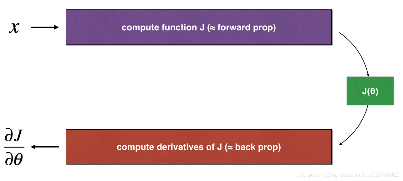
Consider a 1D linear function J(θ)=θxJ(θ)=θx. The model contains only a single real-valued parameter θθ, and takes xx as input.
You will implement code to compute J(.)J(.) and its derivative ∂J∂θ∂J∂θ. You will then use gradient checking to make sure your derivative computation for JJ is correct.

The diagram above shows the key computation steps: First start with xx, then evaluate the function J(x)J(x) ("forward propagation"). Then compute the derivative ∂J∂θ∂J∂θ ("backward propagation").
Exercise: implement "forward propagation" and "backward propagation" for this simple function. I.e., compute both J(.)J(.) ("forward propagation") and its derivative with respect to θθ ("backward propagation"), in two separate functions.
# GRADED FUNCTION: forward_propagation
def forward_propagation(x, theta):
"""
Implement the linear forward propagation (compute J) presented in Figure 1 (J(theta) = theta * x)
Arguments:
x -- a real-valued input
theta -- our parameter, a real number as well
Returns:
J -- the value of function J, computed using the formula J(theta) = theta * x
"""
### START CODE HERE ### (approx. 1 line)
J = theta*x
### END CODE HERE ###
return J
x, theta = 2, 4
J = forward_propagation(x, theta)
print ("J = " + str(J))
Expected Output:
| J | 8 |
Exercise: Now, implement the backward propagation step (derivative computation) of Figure 1. That is, compute the derivative of J(θ)=θxJ(θ)=θx with respect to θθ. To save you from doing the calculus, you should get dtheta=∂J∂θ=xdtheta=∂J∂θ=x.
# GRADED FUNCTION: backward_propagation
def backward_propagation(x, theta):
"""
Computes the derivative of J with respect to theta (see Figure 1).
Arguments:
x -- a real-valued input
theta -- our parameter, a real number as well
Returns:
dtheta -- the gradient of the cost with respect to theta
"""
### START CODE HERE ### (approx. 1 line)
dtheta = x
### END CODE HERE ###
return dtheta
x, theta = 2, 4
dtheta = backward_propagation(x, theta)
print ("dtheta = " + str(dtheta))
Expected Output:
| dtheta | 2 |
Exercise: To show that the backward_propagation() function is correctly computing the gradient ∂J∂θ∂J∂θ, let's implement gradient checking.
Instructions:
- First compute "gradapprox" using the formula above (1) and a small value of εε. Here are the Steps to follow:
- θ+=θ+εθ+=θ+ε
- θ−=θ−εθ−=θ−ε
- J+=J(θ+)J+=J(θ+)
- J−=J(θ−)J−=J(θ−)
- gradapprox=J+−J−2εgradapprox=J+−J−2ε
- Then compute the gradient using backward propagation, and store the result in a variable "grad"
- Finally, compute the relative difference between "gradapprox" and the "grad" using the following formula:
difference=∣∣grad−gradapprox∣∣2∣∣grad∣∣2+∣∣gradapprox∣∣2(2)(2)difference=∣∣grad−gradapprox∣∣2∣∣grad∣∣2+∣∣gradapprox∣∣2You will need 3 Steps to compute this formula:
- 1'. compute the numerator using np.linalg.norm(...)
- 2'. compute the denominator. You will need to call np.linalg.norm(...) twice.
- 3'. divide them.
- If this difference is small (say less than 10−710−7), you can be quite confident that you have computed your gradient correctly. Otherwise, there may be a mistake in the gradient computation.
# GRADED FUNCTION: gradient_check
def gradient_check(x, theta, epsilon = 1e-7):
"""
Implement the backward propagation presented in Figure 1.
Arguments:
x -- a real-valued input
theta -- our parameter, a real number as well
epsilon -- tiny shift to the input to compute approximated gradient with formula(1)
Returns:
difference -- difference (2) between the approximated gradient and the backward propagation gradient
"""
# Compute gradapprox using left side of formula (1). epsilon is small enough, you don't need to worry about the limit.
### START CODE HERE ### (approx. 5 lines)
thetaplus =theta+epsilon # Step 1
thetaminus =theta-epsilon # Step 2
J_plus = forward_propagation(x, thetaplus) # Step 3
J_minus = forward_propagation(x, thetaminus) # Step 4
gradapprox = (J_plus-J_minus)/(2*epsilon) # Step 5
### END CODE HERE ###
# Check if gradapprox is close enough to the output of backward_propagation()
### START CODE HERE ### (approx. 1 line)
grad = backward_propagation(x, theta)
### END CODE HERE ###
### START CODE HERE ### (approx. 1 line)
numerator = np.linalg.norm(grad-gradapprox) # Step 1'
denominator = np.linalg.norm(grad)+np.linalg.norm(gradapprox) # Step 2'
difference = numerator/denominator # Step 3'
### END CODE HERE ###
if difference < 1e-7:
print ("The gradient is correct!")
else:
print ("The gradient is wrong!")
return difference
x, theta = 2, 4
difference = gradient_check(x, theta)
print("difference = " + str(difference))
Expected Output: The gradient is correct!
| difference | 2.9193358103083e-10 |
Congrats, the difference is smaller than the 10−710−7 threshold. So you can have high confidence that you've correctly computed the gradient in backward_propagation().
Now, in the more general case, your cost function JJ has more than a single 1D input. When you are training a neural network, θθ actually consists of multiple matrices W[l]W[l] and biases b[l]b[l]! It is important to know how to do a gradient check with higher-dimensional inputs. Let's do it!
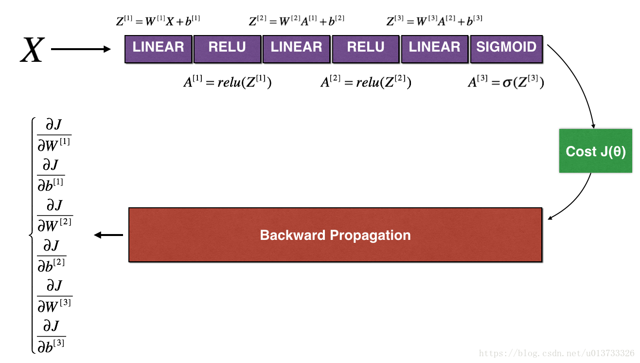
3) N-dimensional gradient checking
The following figure describes the forward and backward propagation of your fraud detection model.

LINEAR -> RELU -> LINEAR -> RELU -> LINEAR -> SIGMOID
Let's look at your implementations for forward propagation and backward propagation.
def forward_propagation_n(X, Y, parameters):
"""
Implements the forward propagation (and computes the cost) presented in Figure 3.
Arguments:
X -- training set for m examples
Y -- labels for m examples
parameters -- python dictionary containing your parameters "W1", "b1", "W2", "b2", "W3", "b3":
W1 -- weight matrix of shape (5, 4)
b1 -- bias vector of shape (5, 1)
W2 -- weight matrix of shape (3, 5)
b2 -- bias vector of shape (3, 1)
W3 -- weight matrix of shape (1, 3)
b3 -- bias vector of shape (1, 1)
Returns:
cost -- the cost function (logistic cost for one example)
"""
# retrieve parameters
m = X.shape[1]
W1 = parameters["W1"]
b1 = parameters["b1"]
W2 = parameters["W2"]
b2 = parameters["b2"]
W3 = parameters["W3"]
b3 = parameters["b3"]
# LINEAR -> RELU -> LINEAR -> RELU -> LINEAR -> SIGMOID
Z1 = np.dot(W1, X) + b1
A1 = relu(Z1)
Z2 = np.dot(W2, A1) + b2
A2 = relu(Z2)
Z3 = np.dot(W3, A2) + b3
A3 = sigmoid(Z3)
# Cost
logprobs = np.multiply(-np.log(A3),Y) + np.multiply(-np.log(1 - A3), 1 - Y)
cost = 1./m * np.sum(logprobs)
cache = (Z1, A1, W1, b1, Z2, A2, W2, b2, Z3, A3, W3, b3)
return cost, cache
Now, run backward propagation.
def backward_propagation_n(X, Y, cache):
"""
Implement the backward propagation presented in figure 2.
Arguments:
X -- input datapoint, of shape (input size, 1)
Y -- true "label"
cache -- cache output from forward_propagation_n()
Returns:
gradients -- A dictionary with the gradients of the cost with respect to each parameter, activation and pre-activation variables.
"""
m = X.shape[1]
(Z1, A1, W1, b1, Z2, A2, W2, b2, Z3, A3, W3, b3) = cache
dZ3 = A3 - Y
dW3 = 1./m * np.dot(dZ3, A2.T)
db3 = 1./m * np.sum(dZ3, axis=1, keepdims = True)
dA2 = np.dot(W3.T, dZ3)
dZ2 = np.multiply(dA2, np.int64(A2 > 0))
dW2 = 1./m * np.dot(dZ2, A1.T)
db2 = 1./m * np.sum(dZ2, axis=1, keepdims = True)
dA1 = np.dot(W2.T, dZ2)
dZ1 = np.multiply(dA1, np.int64(A1 > 0))
dW1 = 1./m * np.dot(dZ1, X.T)
db1 = 1./m * np.sum(dZ1, axis=1, keepdims = True)
gradients = {"dZ3": dZ3, "dW3": dW3, "db3": db3,
"dA2": dA2, "dZ2": dZ2, "dW2": dW2, "db2": db2,
"dA1": dA1, "dZ1": dZ1, "dW1": dW1, "db1": db1}
return gradients
You obtained some results on the fraud detection test set but you are not 100% sure of your model. Nobody's perfect! Let's implement gradient checking to verify if your gradients are correct.
How does gradient checking work?.
As in 1) and 2), you want to compare "gradapprox" to the gradient computed by backpropagation. The formula is still:
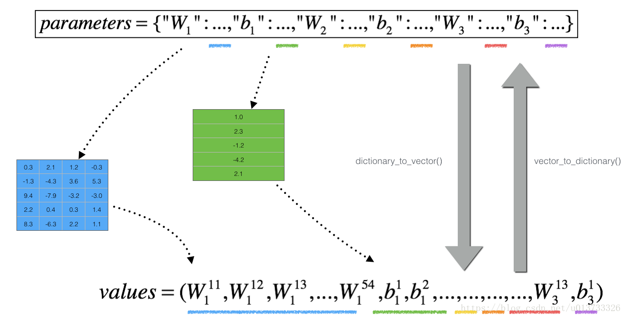
However, θθ is not a scalar anymore. It is a dictionary called "parameters". We implemented a function "dictionary_to_vector()" for you. It converts the "parameters" dictionary into a vector called "values", obtained by reshaping all parameters (W1, b1, W2, b2, W3, b3) into vectors and concatenating them.
The inverse function is "vector_to_dictionary" which outputs back the "parameters" dictionary.

You will need these functions in gradient_check_n()
We have also converted the "gradients" dictionary into a vector "grad" using gradients_to_vector(). You don't need to worry about that.
Exercise: Implement gradient_check_n().
Instructions: Here is pseudo-code that will help you implement the gradient check.
For each i in num_parameters:
- To compute
J_plus[i]:- Set θ+θ+ to
np.copy(parameters_values) - Set θ+iθi+ to θ+i+εθi++ε
- Calculate J+iJi+ using to
forward_propagation_n(x, y, vector_to_dictionary(θ+θ+)).
- Set θ+θ+ to
- To compute
J_minus[i]: do the same thing with θ−θ− - Compute gradapprox[i]=J+i−J−i2εgradapprox[i]=Ji+−Ji−2ε
Thus, you get a vector gradapprox, where gradapprox[i] is an approximation of the gradient with respect to parameter_values[i]. You can now compare this gradapprox vector to the gradients vector from backpropagation. Just like for the 1D case (Steps 1', 2', 3'), compute:
# GRADED FUNCTION: gradient_check_n
def gradient_check_n(parameters, gradients, X, Y, epsilon = 1e-7):
"""
Checks if backward_propagation_n computes correctly the gradient of the cost output by forward_propagation_n
Arguments:
parameters -- python dictionary containing your parameters "W1", "b1", "W2", "b2", "W3", "b3":
grad -- output of backward_propagation_n, contains gradients of the cost with respect to the parameters.
x -- input datapoint, of shape (input size, 1)
y -- true "label"
epsilon -- tiny shift to the input to compute approximated gradient with formula(1)
Returns:
difference -- difference (2) between the approximated gradient and the backward propagation gradient
"""
# Set-up variables
parameters_values, _ = dictionary_to_vector(parameters)
grad = gradients_to_vector(gradients)
num_parameters = parameters_values.shape[0]
J_plus = np.zeros((num_parameters, 1))
J_minus = np.zeros((num_parameters, 1))
gradapprox = np.zeros((num_parameters, 1))
# Compute gradapprox
for i in range(num_parameters):
# Compute J_plus[i]. Inputs: "parameters_values, epsilon". Output = "J_plus[i]".
# "_" is used because the function you have to outputs two parameters but we only care about the first one
### START CODE HERE ### (approx. 3 lines)
thetaplus = np.copy(parameters_values) # Step 1
thetaplus[i][0] =thetaplus[i][0]+epsilon # Step 2
J_plus[i], _ = forward_propagation_n(X, Y, vector_to_dictionary( thetaplus)) # Step 3
### END CODE HERE ###
# Compute J_minus[i]. Inputs: "parameters_values, epsilon". Output = "J_minus[i]".
### START CODE HERE ### (approx. 3 lines)
thetaminus = np.copy(parameters_values) # Step 1
thetaminus[i][0] = thetaminus[i][0]-epsilon # Step 2
J_minus[i], _ = forward_propagation_n(X, Y, vector_to_dictionary( thetaminus )) # Step 3
### END CODE HERE ###
# Compute gradapprox[i]
### START CODE HERE ### (approx. 1 line)
gradapprox[i] =(J_plus[i] -J_minus[i])/(2*epsilon)
### END CODE HERE ###
# Compare gradapprox to backward propagation gradients by computing difference.
### START CODE HERE ### (approx. 1 line)
numerator = np.linalg.norm(grad-gradapprox) # Step 1'
denominator =np.linalg.norm(grad)+ np.linalg.norm(gradapprox) # Step 2'
difference = numerator/denominator # Step 3'
### END CODE HERE ###
if difference > 2e-7:
print ("\033[93m" + "There is a mistake in the backward propagation! difference = " + str(difference) + "\033[0m")
else:
print ("\033[92m" + "Your backward propagation works perfectly fine! difference = " + str(difference) + "\033[0m")
return difference
X, Y, parameters = gradient_check_n_test_case()
cost, cache = forward_propagation_n(X, Y, parameters)
gradients = backward_propagation_n(X, Y, cache)
difference = gradient_check_n(parameters, gradients, X, Y)
Expected output:
| There is a mistake in the backward propagation! | difference = 0.285093156781 |
It seems that there were errors in the backward_propagation_n code we gave you! Good that you've implemented the gradient check. Go back to backward_propagation and try to find/correct the errors (Hint: check dW2 and db1). Rerun the gradient check when you think you've fixed it. Remember you'll need to re-execute the cell defining backward_propagation_n() if you modify the code.
Can you get gradient check to declare your derivative computation correct? Even though this part of the assignment isn't graded, we strongly urge you to try to find the bug and re-run gradient check until you're convinced backprop is now correctly implemented.
Note
- Gradient Checking is slow! Approximating the gradient with ∂J∂θ≈J(θ+ε)−J(θ−ε)2ε∂J∂θ≈J(θ+ε)−J(θ−ε)2ε is computationally costly. For this reason, we don't run gradient checking at every iteration during training. Just a few times to check if the gradient is correct.
- Gradient Checking, at least as we've presented it, doesn't work with dropout. You would usually run the gradient check algorithm without dropout to make sure your backprop is correct, then add dropout.
Congrats, you can be confident that your deep learning model for fraud detection is working correctly! You can even use this to convince your CEO. :)
What you should remember from this notebook:
- Gradient checking verifies closeness between the gradients from backpropagation and the numerical approximation of the gradient (computed using forward propagation).
- Gradient checking is slow, so we don't run it in every iteration of training. You would usually run it only to make sure your code is correct, then turn it off and use backprop for the actual learning process.
找的其他人的中文版-----------------------------------------------------------------------------------------------------------------------------------------------------------------------------
梯度校验
You are part of a team working to make mobile payments available globally, and are asked to build a deep learning model to detect fraud–whenever someone makes a payment, you want to see if the payment might be fraudulent, such as if the user’s account has been taken over by a hacker.
But backpropagation is quite challenging to implement, and sometimes has bugs. Because this is a mission-critical application, your company’s CEO wants to be really certain that your implementation of backpropagation is correct. Your CEO says, “Give me a proof that your backpropagation is actually working!” To give this reassurance, you are going to use “gradient checking”.
假设你现在是一个全球移动支付团队中的一员,现在需要建立一个深度学习模型去判断用户账户在进行付款的时候是否是被黑客入侵的。
但是,在我们执行反向传播的计算过程中,反向传播函数的计算过程是比较复杂的。为了验证我们得到的反向传播函数是否正确,现在你需要编写一些代码来验证反向传播函数的正确性。
反向传播计算梯度 ∂J∂θ∂J∂θ, θθ表示模型中的参数,使用前向传播和损失函数计算 JJ,因为向前传播相对容易实现,所以您确信自己得到了正确的结果,所以您几乎100%确定您正确计算了 JJ的成本。 因此,您可以使用您的代码来计算 JJ来验证计算的代码∂J∂θ∂J∂θ。
让我们回头看一下导数(或梯度)的定义:
- ∂J∂θ∂J∂θ 是你想确保你的计算正确的值。
- 你可以计算 J(θ+ε)J(θ+ε) 和 J(θ−ε)J(θ−ε) (在θθ是一个实数的情况下),因为你确信你对JJ的实现是正确的。
我们先来看一下一维线性模型的梯度检查计算过程:
一维线性
def forward_propagation(x,theta):
""" 实现图中呈现的线性前向传播(计算J)(J(theta)= theta * x) 参数: x - 一个实值输入 theta - 参数,也是一个实数 返回: J - 函数J的值,用公式J(theta)= theta * x计算 """ J = np.dot(theta,x) return J- 1
- 2
- 3
- 4
- 5
- 6
- 7
- 8
- 9
- 10
- 11
- 12
- 13
- 14
- 15
测试一下:
#测试forward_propagation
print("-----------------测试forward_propagation-----------------")
x, theta = 2, 4
J = forward_propagation(x, theta)
print ("J = " + str(J))- 1
- 2
- 3
- 4
- 5
测试结果:
-----------------测试forward_propagation-----------------
J = 8- 1
- 2
前向传播有了,我们来看一下反向传播:
def backward_propagation(x,theta):
""" 计算J相对于θ的导数。 参数: x - 一个实值输入 theta - 参数,也是一个实数 返回: dtheta - 相对于θ的成本梯度 """ dtheta = x return dtheta- 1
- 2
- 3
- 4
- 5
- 6
- 7
- 8
- 9
- 10
- 11
- 12
- 13
- 14
测试一下:
#测试backward_propagation
print("-----------------测试backward_propagation-----------------")
x, theta = 2, 4
dtheta = backward_propagation(x, theta)
print ("dtheta = " + str(dtheta))- 1
- 2
- 3
- 4
- 5
测试结果:
-----------------测试backward_propagation-----------------
dtheta = 2- 1
- 2
梯度检查的步骤如下:
- θ+=θ+εθ+=θ+ε
- θ−=θ−εθ−=θ−ε
- J+=J(θ+)J+=J(θ+)
- J−=J(θ−)J−=J(θ−)
- gradapprox=J+−J−2εgradapprox=J+−J−2ε
接下来,计算梯度的反向传播值,最后计算误差:
当difference小于10−710−7时,我们通常认为我们计算的结果是正确的。
def gradient_check(x,theta,epsilon=1e-7): """ 实现图中的反向传播。 参数: x - 一个实值输入 theta - 参数,也是一个实数 epsilon - 使用公式(3)计算输入的微小偏移以计算近似梯度 返回: 近似梯度和后向传播梯度之间的差异 """ #使用公式(3)的左侧计算gradapprox。 thetaplus = theta + epsilon # Step 1 thetaminus = theta - epsilon # Step 2 J_plus = forward_propagation(x, thetaplus) # Step 3 J_minus = forward_propagation(x, thetaminus) # Step 4 gradapprox = (J_plus - J_minus) / (2 * epsilon) # Step 5 #检查gradapprox是否足够接近backward_propagation()的输出 grad = backward_propagation(x, theta) numerator = np.linalg.norm(grad - gradapprox) # Step 1' denominator = np.linalg.norm(grad) + np.linalg.norm(gradapprox) # Step 2' difference = numerator / denominator # Step 3' if difference < 1e-7: print("梯度检查:梯度正常!") else: print("梯度检查:梯度超出阈值!") return difference- 1
- 2
- 3
- 4
- 5
- 6
- 7
- 8
- 9
- 10
- 11
- 12
- 13
- 14
- 15
- 16
- 17
- 18
- 19
- 20
- 21
- 22
- 23
- 24
- 25
- 26
- 27
- 28
- 29
- 30
- 31
- 32
- 33
- 34
- 35
测试一下:
#测试gradient_check
print("-----------------测试gradient_check-----------------")
x, theta = 2, 4
difference = gradient_check(x, theta)
print("difference = " + str(difference))- 1
- 2
- 3
- 4
- 5
测试结果:
-----------------测试gradient_check-----------------
梯度检查:梯度正常!
difference = 2.91933588329e-10- 1
- 2
- 3
高维参数是怎样计算的呢?我们看一下下图:
高维
def forward_propagation_n(X,Y,parameters):
""" 实现图中的前向传播(并计算成本)。 参数: X - 训练集为m个例子 Y - m个示例的标签 parameters - 包含参数“W1”,“b1”,“W2”,“b2”,“W3”,“b3”的python字典: W1 - 权重矩阵,维度为(5,4) b1 - 偏向量,维度为(5,1) W2 - 权重矩阵,维度为(3,5) b2 - 偏向量,维度为(3,1) W3 - 权重矩阵,维度为(1,3) b3 - 偏向量,维度为(1,1) 返回: cost - 成本函数(logistic) """ m = X.shape[1] W1 = parameters["W1"] b1 = parameters["b1"] W2 = parameters["W2"] b2 = parameters["b2"] W3 = parameters["W3"] b3 = parameters["b3"] # LINEAR -> RELU -> LINEAR -> RELU -> LINEAR -> SIGMOID Z1 = np.dot(W1,X) + b1 A1 = gc_utils.relu(Z1) Z2 = np.dot(W2,A1) + b2 A2 = gc_utils.relu(Z2) Z3 = np.dot(W3,A2) + b3 A3 = gc_utils.sigmoid(Z3) #计算成本 logprobs = np.multiply(-np.log(A3), Y) + np.multiply(-np.log(1 - A3), 1 - Y) cost = (1 / m) * np.sum(logprobs) cache = (Z1, A1, W1, b1, Z2, A2, W2, b2, Z3, A3, W3, b3) return cost, cache def backward_propagation_n(X,Y,cache): """ 实现图中所示的反向传播。 参数: X - 输入数据点(输入节点数量,1) Y - 标签 cache - 来自forward_propagation_n()的cache输出 返回: gradients - 一个字典,其中包含与每个参数、激活和激活前变量相关的成本梯度。 """ m = X.shape[1] (Z1, A1, W1, b1, Z2, A2, W2, b2, Z3, A3, W3, b3) = cache dZ3 = A3 - Y dW3 = (1. / m) * np.dot(dZ3,A2.T) dW3 = 1. / m * np.dot(dZ3, A2.T) db3 = 1. / m * np.sum(dZ3, axis=1, keepdims=True) dA2 = np.dot(W3.T, dZ3) dZ2 = np.multiply(dA2, np.int64(A2 > 0)) #dW2 = 1. / m * np.dot(dZ2, A1.T) * 2 # Should not multiply by 2 dW2 = 1. / m * np.dot(dZ2, A1.T) db2 = 1. / m * np.sum(dZ2, axis=1, keepdims=True) dA1 = np.dot(W2.T, dZ2) dZ1 = np.multiply(dA1, np.int64(A1 > 0)) dW1 = 1. / m * np.dot(dZ1, X.T) #db1 = 4. / m * np.sum(dZ1, axis=1, keepdims=True) # Should not multiply by 4 db1 = 1. / m * np.sum(dZ1, axis=1, keepdims=True) gradients = {"dZ3": dZ3, "dW3": dW3, "db3": db3, "dA2": dA2, "dZ2": dZ2, "dW2": dW2, "db2": db2, "dA1": dA1, "dZ1": dZ1, "dW1": dW1, "db1": db1} return gradients - 1
- 2
- 3
- 4
- 5
- 6
- 7
- 8
- 9
- 10
- 11
- 12
- 13
- 14
- 15
- 16
- 17
- 18
- 19
- 20
- 21
- 22
- 23
- 24
- 25
- 26
- 27
- 28
- 29
- 30
- 31
- 32
- 33
- 34
- 35
- 36
- 37
- 38
- 39
- 40
- 41
- 42
- 43
- 44
- 45
- 46
- 47
- 48
- 49
- 50
- 51
- 52
- 53
- 54
- 55
- 56
- 57
- 58
- 59
- 60
- 61
- 62
- 63
- 64
- 65
- 66
- 67
- 68
- 69
- 70
- 71
- 72
- 73
- 74
- 75
- 76
- 77
- 78
- 79
- 80
- 81
- 82
如果想比较“gradapprox”与反向传播计算的梯度。 该公式仍然是:
∂J∂θ=limε→0J(θ+ε)−J(θ−ε)2ε(3)(3)∂J∂θ=limε→0J(θ+ε)−J(θ−ε)2ε
然而,θθ不再是标量。 这是一个名为“parameters”的字典。 我们为你实现了一个函数“dictionary_to_vector()”。 它将“parameters”字典转换为一个称为“values”的向量,通过将所有参数(W1,b1,W2,b2,W3,b3)整形为向量并将它们连接起来而获得。
反函数是“vector_to_dictionary”,它返回“parameters”字典。
这里是伪代码,可以帮助你实现梯度检查:
For i in num_parameters:
- 计算
J_plus[i]:
- 把 θ+θ+ 设置为
np.copy(parameters_values) - 把 θ+iθi+ 设置为 θ+i+εθi++ε
- 使用
forward_propagation_n(x, y, vector_to_dictionary(θ+θ+))来计算J+iJi+
- 把 θ+θ+ 设置为
- 计算
J_minus[i]: 使用相同的方法计算 θ−θ− - 计算gradapprox[i]=J+i−J−i2εgradapprox[i]=Ji+−Ji−2ε
- 计算梯度
- 计算误差:
difference=∥grad−gradapprox∥2∥grad∥2+∥gradapprox∥2(4)(4)difference=‖grad−gradapprox‖2‖grad‖2+‖gradapprox‖2
def gradient_check_n(parameters,gradients,X,Y,epsilon=1e-7): """ 检查backward_propagation_n是否正确计算forward_propagation_n输出的成本梯度 参数: parameters - 包含参数“W1”,“b1”,“W2”,“b2”,“W3”,“b3”的python字典: grad_output_propagation_n的输出包含与参数相关的成本梯度。 x - 输入数据点,维度为(输入节点数量,1) y - 标签 epsilon - 计算输入的微小偏移以计算近似梯度 返回: difference - 近似梯度和后向传播梯度之间的差异 """ #初始化参数 parameters_values , keys = gc_utils.dictionary_to_vector(parameters) #keys用不到 grad = gc_utils.gradients_to_vector(gradients) num_parameters = parameters_values.shape[0] J_plus = np.zeros((num_parameters,1)) J_minus = np.zeros((num_parameters,1)) gradapprox = np.zeros((num_parameters,1)) #计算gradapprox for i in range(num_parameters): #计算J_plus [i]。输入:“parameters_values,epsilon”。输出=“J_plus [i]” thetaplus = np.copy(parameters_values) # Step 1 thetaplus[i][0] = thetaplus[i][0] + epsilon # Step 2 J_plus[i], cache = forward_propagation_n(X,Y,gc_utils.vector_to_dictionary(thetaplus)) # Step 3 ,cache用不到 #计算J_minus [i]。输入:“parameters_values,epsilon”。输出=“J_minus [i]”。 thetaminus = np.copy(parameters_values) # Step 1 thetaminus[i][0] = thetaminus[i][0] - epsilon # Step 2 J_minus[i], cache = forward_propagation_n(X,Y,gc_utils.vector_to_dictionary(thetaminus))# Step 3 ,cache用不到 #计算gradapprox[i] gradapprox[i] = (J_plus[i] - J_minus[i]) / (2 * epsilon) #通过计算差异比较gradapprox和后向传播梯度。 numerator = np.linalg.norm(grad - gradapprox) # Step 1' denominator = np.linalg.norm(grad) + np.linalg.norm(gradapprox) # Step 2' difference = numerator / denominator # Step 3' if difference < 1e-7: print("梯度检查:梯度正常!") else: print("梯度检查:梯度超出阈值!") return difference到此为止,这篇博文就算完成了,因为我没有弄到testCase.py,所以最后这一点点的梯度检查没法做,由此带来的麻烦还望多多谅解。
相关库代码
init_utils.py
# -*- coding: utf-8 -*-

#init_utils.py

import numpy as np
import matplotlib.pyplot as plt import sklearn import sklearn.datasets def sigmoid(x): """ Compute the sigmoid of x Arguments: x -- A scalar or numpy array of any size. Return: s -- sigmoid(x) """ s = 1/(1+np.exp(-x)) return s def relu(x): """ Compute the relu of x Arguments: x -- A scalar or numpy array of any size. Return: s -- relu(x) """ s = np.maximum(0,x) return s def compute_loss(a3, Y): """ Implement the loss function Arguments: a3 -- post-activation, output of forward propagation Y -- "true" labels vector, same shape as a3 Returns: loss - value of the loss function """ m = Y.shape[1] logprobs = np.multiply(-np.log(a3),Y) + np.multiply(-np.log(1 - a3), 1 - Y) loss = 1./m * np.nansum(logprobs) return loss def forward_propagation(X, parameters): """ Implements the forward propagation (and computes the loss) presented in Figure 2. Arguments: X -- input dataset, of shape (input size, number of examples) Y -- true "label" vector (containing 0 if cat, 1 if non-cat) parameters -- python dictionary containing your parameters "W1", "b1", "W2", "b2", "W3", "b3": W1 -- weight matrix of shape () b1 -- bias vector of shape () W2 -- weight matrix of shape () b2 -- bias vector of shape () W3 -- weight matrix of shape () b3 -- bias vector of shape () Returns: loss -- the loss function (vanilla logistic loss) """ # retrieve parameters W1 = parameters["W1"] b1 = parameters["b1"] W2 = parameters["W2"] b2 = parameters["b2"] W3 = parameters["W3"] b3 = parameters["b3"] # LINEAR -> RELU -> LINEAR -> RELU -> LINEAR -> SIGMOID z1 = np.dot(W1, X) + b1 a1 = relu(z1) z2 = np.dot(W2, a1) + b2 a2 = relu(z2) z3 = np.dot(W3, a2) + b3 a3 = sigmoid(z3) cache = (z1, a1, W1, b1, z2, a2, W2, b2, z3, a3, W3, b3) return a3, cache def backward_propagation(X, Y, cache): """ Implement the backward propagation presented in figure 2. Arguments: X -- input dataset, of shape (input size, number of examples) Y -- true "label" vector (containing 0 if cat, 1 if non-cat) cache -- cache output from forward_propagation() Returns: gradients -- A dictionary with the gradients with respect to each parameter, activation and pre-activation variables """ m = X.shape[1] (z1, a1, W1, b1, z2, a2, W2, b2, z3, a3, W3, b3) = cache dz3 = 1./m * (a3 - Y) dW3 = np.dot(dz3, a2.T) db3 = np.sum(dz3, axis=1, keepdims = True) da2 = np.dot(W3.T, dz3) dz2 = np.multiply(da2, np.int64(a2 > 0)) dW2 = np.dot(dz2, a1.T) db2 = np.sum(dz2, axis=1, keepdims = True) da1 = np.dot(W2.T, dz2) dz1 = np.multiply(da1, np.int64(a1 > 0)) dW1 = np.dot(dz1, X.T) db1 = np.sum(dz1, axis=1, keepdims = True) gradients = {"dz3": dz3, "dW3": dW3, "db3": db3, "da2": da2, "dz2": dz2, "dW2": dW2, "db2": db2, "da1": da1, "dz1": dz1, "dW1": dW1, "db1": db1} return gradients def update_parameters(parameters, grads, learning_rate): """ Update parameters using gradient descent Arguments: parameters -- python dictionary containing your parameters grads -- python dictionary containing your gradients, output of n_model_backward Returns: parameters -- python dictionary containing your updated parameters parameters['W' + str(i)] = ... parameters['b' + str(i)] = ... """ L = len(parameters) // 2 # number of layers in the neural networks # Update rule for each parameter for k in range(L): parameters["W" + str(k+1)] = parameters["W" + str(k+1)] - learning_rate * grads["dW" + str(k+1)] parameters["b" + str(k+1)] = parameters["b" + str(k+1)] - learning_rate * grads["db" + str(k+1)] return parameters def predict(X, y, parameters): """ This function is used to predict the results of a n-layer neural network. Arguments: X -- data set of examples you would like to label parameters -- parameters of the trained model Returns: p -- predictions for the given dataset X """ m = X.shape[1] p = np.zeros((1,m), dtype = np.int) # Forward propagation a3, caches = forward_propagation(X, parameters) # convert probas to 0/1 predictions for i in range(0, a3.shape[1]): if a3[0,i] > 0.5: p[0,i] = 1 else: p[0,i] = 0 # print results print("Accuracy: " + str(np.mean((p[0,:] == y[0,:])))) return p def load_dataset(is_plot=True): np.random.seed(1) train_X, train_Y = sklearn.datasets.make_circles(n_samples=300, noise=.05) np.random.seed(2) test_X, test_Y = sklearn.datasets.make_circles(n_samples=100, noise=.05) # Visualize the data if is_plot: plt.scatter(train_X[:, 0], train_X[:, 1], c=train_Y, s=40, cmap=plt.cm.Spectral); train_X = train_X.T train_Y = train_Y.reshape((1, train_Y.shape[0])) test_X = test_X.T test_Y = test_Y.reshape((1, test_Y.shape[0])) return train_X, train_Y, test_X, test_Y def plot_decision_boundary(model, X, y): # Set min and max values and give it some padding x_min, x_max = X[0, :].min() - 1, X[0, :].max() + 1 y_min, y_max = X[1, :].min() - 1, X[1, :].max() + 1 h = 0.01 # Generate a grid of points with distance h between them xx, yy = np.meshgrid(np.arange(x_min, x_max, h), np.arange(y_min, y_max, h)) # Predict the function value for the whole grid Z = model(np.c_[xx.ravel(), yy.ravel()]) Z = Z.reshape(xx.shape) # Plot the contour and training examples plt.contourf(xx, yy, Z, cmap=plt.cm.Spectral) plt.ylabel('x2') plt.xlabel('x1') plt.scatter(X[0, :], X[1, :], c=y, cmap=plt.cm.Spectral) plt.show() def predict_dec(parameters, X): """ Used for plotting decision boundary. Arguments: parameters -- python dictionary containing your parameters X -- input data of size (m, K) Returns predictions -- vector of predictions of our model (red: 0 / blue: 1) """ # Predict using forward propagation and a classification threshold of 0.5 a3, cache = forward_propagation(X, parameters) predictions = (a3>0.5) return predictions
gc_utils.py
# -*- coding: utf-8 -*-

#gc_utils.py

import numpy as np
import matplotlib.pyplot as plt def sigmoid(x): """ Compute the sigmoid of x Arguments: x -- A scalar or numpy array of any size. Return: s -- sigmoid(x) """ s = 1/(1+np.exp(-x)) return s def relu(x): """ Compute the relu of x Arguments: x -- A scalar or numpy array of any size. Return: s -- relu(x) """ s = np.maximum(0,x) return s def dictionary_to_vector(parameters): """ Roll all our parameters dictionary into a single vector satisfying our specific required shape. """ keys = [] count = 0 for key in ["W1", "b1", "W2", "b2", "W3", "b3"]: # flatten parameter new_vector = np.reshape(parameters[key], (-1,1)) keys = keys + [key]*new_vector.shape[0] if count == 0: theta = new_vector else: theta = np.concatenate((theta, new_vector), axis=0) count = count + 1 return theta, keys def vector_to_dictionary(theta): """ Unroll all our parameters dictionary from a single vector satisfying our specific required shape. """ parameters = {} parameters["W1"] = theta[:20].reshape((5,4)) parameters["b1"] = theta[20:25].reshape((5,1)) parameters["W2"] = theta[25:40].reshape((3,5)) parameters["b2"] = theta[40:43].reshape((3,1)) parameters["W3"] = theta[43:46].reshape((1,3)) parameters["b3"] = theta[46:47].reshape((1,1)) return parameters def gradients_to_vector(gradients): """ Roll all our gradients dictionary into a single vector satisfying our specific required shape. """ count = 0 for key in ["dW1", "db1", "dW2", "db2", "dW3", "db3"]: # flatten parameter new_vector = np.reshape(gradients[key], (-1,1)) if count == 0: theta = new_vector else: theta = np.concatenate((theta, new_vector), axis=0) count = count + 1 return theta