import numpy as np
import matplotlib.pyplot as plt
import sklearn
import sklearn.datasets
import init_utils   #第一部分，初始化
import reg_utils    #第二部分，正则化
import gc_utils     #第三部分，梯度校验
#%matplotlib inline #如果你使用的是Jupyter Notebook，请取消注释。
plt.rcParams['figure.figsize'] = (7.0, 4.0) # set default size of plots
plt.rcParams['image.interpolation'] = 'nearest'
plt.rcParams['image.cmap'] = 'gray'

2.1 数据

train_X, train_Y, test_X, test_Y = init_utils.load_dataset(is_plot=True)

在这里插入图片描述

2.2 神经网络模型

def model(X,Y,learning_rate=0.01,num_iterations=15000,print_cost=True,initialization="he",is_polt=True):
    """
    实现一个三层的神经网络：LINEAR ->RELU -> LINEAR -> RELU -> LINEAR -> SIGMOID

    参数：
        X - 输入的数据，维度为(2, 要训练/测试的数量)
        Y - 标签，【0 | 1】，维度为(1，对应的是输入的数据的标签)
        learning_rate - 学习速率
        num_iterations - 迭代的次数
        print_cost - 是否打印成本值，每迭代1000次打印一次
        initialization - 字符串类型，初始化的类型【"zeros" | "random" | "he"】
        is_polt - 是否绘制梯度下降的曲线图
    返回
        parameters - 学习后的参数
    """
    grads = {}
    costs = []
    m = X.shape[1]
    layers_dims = [X.shape[0],10,5,1]

    #选择初始化参数的类型
    if initialization == "zeros":
        parameters = initialize_parameters_zeros(layers_dims)
    elif initialization == "random":
        parameters = initialize_parameters_random(layers_dims)
    elif initialization == "he":
        parameters = initialize_parameters_he(layers_dims)
    else : 
        print("错误的初始化参数！程序退出")
        exit

    #开始学习
    for i in range(0,num_iterations):
        #前向传播
        a3 , cache = init_utils.forward_propagation(X,parameters)

        #计算成本        
        cost = init_utils.compute_loss(a3,Y)

        #反向传播
        grads = init_utils.backward_propagation(X,Y,cache)

        #更新参数
        parameters = init_utils.update_parameters(parameters,grads,learning_rate)

        #记录成本
        if i % 1000 == 0:
            costs.append(cost)
            #打印成本
            if print_cost:
                print("第" + str(i) + "次迭代，成本值为：" + str(cost))


    #学习完毕，绘制成本曲线
    if is_polt:
        plt.plot(costs)
        plt.ylabel('cost')
        plt.xlabel('iterations (per hundreds)')
        plt.title("Learning rate =" + str(learning_rate))
        plt.show()

    #返回学习完毕后的参数
    return parameters

2.3 初始化为零

2.3.1 代码

def initialize_parameters_zeros(layers_dims):
    """
    将模型的参数全部设置为0

    参数：
        layers_dims - 列表，模型的层数和对应每一层的节点的数量
    返回
        parameters - 包含了所有W和b的字典
            W1 - 权重矩阵，维度为（layers_dims[1], layers_dims[0]）
            b1 - 偏置向量，维度为（layers_dims[1],1）
            ···
            WL - 权重矩阵，维度为（layers_dims[L], layers_dims[L -1]）
            bL - 偏置向量，维度为（layers_dims[L],1）
    """
    parameters = {}

    L = len(layers_dims) #网络层数

    for l in range(1,L):
        parameters["W" + str(l)] = np.zeros((layers_dims[l],layers_dims[l-1]))
        parameters["b" + str(l)] = np.zeros((layers_dims[l],1))

        #使用断言确保我的数据格式是正确的
        assert(parameters["W" + str(l)].shape == (layers_dims[l],layers_dims[l-1]))
        assert(parameters["b" + str(l)].shape == (layers_dims[l],1))

    return parameters

2.3.2 训练

parameters = model(train_X,train_Y,initialization="zeros",is_polt=True)
parameters

第0次迭代，成本值为：0.6931471805599453
第1000次迭代，成本值为：0.6931471805599453
第2000次迭代，成本值为：0.6931471805599453
第3000次迭代，成本值为：0.6931471805599453
第4000次迭代，成本值为：0.6931471805599453
第5000次迭代，成本值为：0.6931471805599453
第6000次迭代，成本值为：0.6931471805599453
第7000次迭代，成本值为：0.6931471805599453
第8000次迭代，成本值为：0.6931471805599453
第9000次迭代，成本值为：0.6931471805599453
第10000次迭代，成本值为：0.6931471805599455
第11000次迭代，成本值为：0.6931471805599453
第12000次迭代，成本值为：0.6931471805599453
第13000次迭代，成本值为：0.6931471805599453
第14000次迭代，成本值为：0.6931471805599453

在这里插入图片描述

{'W1': array([[0., 0.],
        [0., 0.],
        [0., 0.],
        [0., 0.],
        [0., 0.],
        [0., 0.],
        [0., 0.],
        [0., 0.],
        [0., 0.],
        [0., 0.]]), 'W2': array([[0., 0., 0., 0., 0., 0., 0., 0., 0., 0.],
        [0., 0., 0., 0., 0., 0., 0., 0., 0., 0.],
        [0., 0., 0., 0., 0., 0., 0., 0., 0., 0.],
        [0., 0., 0., 0., 0., 0., 0., 0., 0., 0.],
        [0., 0., 0., 0., 0., 0., 0., 0., 0., 0.]]), 'W3': array([[0., 0., 0., 0., 0.]]), 'b1': array([[0.],
        [0.],
        [0.],
        [0.],
        [0.],
        [0.],
        [0.],
        [0.],
        [0.],
        [0.]]), 'b2': array([[0.],
        [0.],
        [0.],
        [0.],
        [0.]]), 'b3': array([[1.6549262e-16]])}

2.3.3 预测

print ("训练集:")
predictions_train = init_utils.predict(train_X, train_Y, parameters)
print ("测试集:")
predictions_test = init_utils.predict(test_X, test_Y, parameters)

训练集:
Accuracy: 0.5
测试集:
Accuracy: 0.5

predictions_train

array([[0, 0, 0, 0, 0, 0, 0, 0, 0, 0, 0, 0, 0, 0, 0, 0, 0, 0, 0, 0, 0, 0,
        0, 0, 0, 0, 0, 0, 0, 0, 0, 0, 0, 0, 0, 0, 0, 0, 0, 0, 0, 0, 0, 0,
        0, 0, 0, 0, 0, 0, 0, 0, 0, 0, 0, 0, 0, 0, 0, 0, 0, 0, 0, 0, 0, 0,
        0, 0, 0, 0, 0, 0, 0, 0, 0, 0, 0, 0, 0, 0, 0, 0, 0, 0, 0, 0, 0, 0,
        0, 0, 0, 0, 0, 0, 0, 0, 0, 0, 0, 0, 0, 0, 0, 0, 0, 0, 0, 0, 0, 0,
        0, 0, 0, 0, 0, 0, 0, 0, 0, 0, 0, 0, 0, 0, 0, 0, 0, 0, 0, 0, 0, 0,
        0, 0, 0, 0, 0, 0, 0, 0, 0, 0, 0, 0, 0, 0, 0, 0, 0, 0, 0, 0, 0, 0,
        0, 0, 0, 0, 0, 0, 0, 0, 0, 0, 0, 0, 0, 0, 0, 0, 0, 0, 0, 0, 0, 0,
        0, 0, 0, 0, 0, 0, 0, 0, 0, 0, 0, 0, 0, 0, 0, 0, 0, 0, 0, 0, 0, 0,
        0, 0, 0, 0, 0, 0, 0, 0, 0, 0, 0, 0, 0, 0, 0, 0, 0, 0, 0, 0, 0, 0,
        0, 0, 0, 0, 0, 0, 0, 0, 0, 0, 0, 0, 0, 0, 0, 0, 0, 0, 0, 0, 0, 0,
        0, 0, 0, 0, 0, 0, 0, 0, 0, 0, 0, 0, 0, 0, 0, 0, 0, 0, 0, 0, 0, 0,
        0, 0, 0, 0, 0, 0, 0, 0, 0, 0, 0, 0, 0, 0, 0, 0, 0, 0, 0, 0, 0, 0,
        0, 0, 0, 0, 0, 0, 0, 0, 0, 0, 0, 0, 0, 0]])

predictions_test

array([[0, 0, 0, 0, 0, 0, 0, 0, 0, 0, 0, 0, 0, 0, 0, 0, 0, 0, 0, 0, 0, 0,
        0, 0, 0, 0, 0, 0, 0, 0, 0, 0, 0, 0, 0, 0, 0, 0, 0, 0, 0, 0, 0, 0,
        0, 0, 0, 0, 0, 0, 0, 0, 0, 0, 0, 0, 0, 0, 0, 0, 0, 0, 0, 0, 0, 0,
        0, 0, 0, 0, 0, 0, 0, 0, 0, 0, 0, 0, 0, 0, 0, 0, 0, 0, 0, 0, 0, 0,
        0, 0, 0, 0, 0, 0, 0, 0, 0, 0, 0, 0]])

可以看到所有预测结果全部预测为0了，所以和瞎猜差不多了，初始化参数为0效果很差！

2.4 随机初始化

2.4.1 代码

def initialize_parameters_random(layers_dims):
    """
    将模型的参数随机初始化

    参数：
        layers_dims - 列表，模型的层数和对应每一层的节点的数量
    返回
        parameters - 包含了所有W和b的字典
            W1 - 权重矩阵，维度为（layers_dims[1], layers_dims[0]）
            b1 - 偏置向量，维度为（layers_dims[1],1）
            ···
            WL - 权重矩阵，维度为（layers_dims[L], layers_dims[L -1]）
            bL - 偏置向量，维度为（layers_dims[L],1）
    """
    np.random.seed(3)               # 指定随机种子
    parameters = {}

    L = len(layers_dims) #网络层数

    for l in range(1,L):
        parameters["W" + str(l)] = np.random.randn(layers_dims[l],layers_dims[l-1]) * 10 # 10倍缩放
        parameters["b" + str(l)] = np.zeros((layers_dims[l],1)) # b无所谓 可以还是初始化为0 

        #使用断言确保我的数据格式是正确的
        assert(parameters["W" + str(l)].shape == (layers_dims[l],layers_dims[l-1]))
        assert(parameters["b" + str(l)].shape == (layers_dims[l],1))

    return parameters

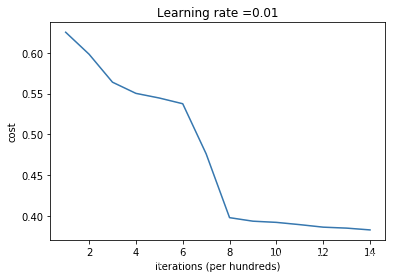
2.4.2 训练

parameters = model(train_X,train_Y,initialization="random",is_polt=True)
parameters

/Users/apple/Desktop/深度学习/课程2-week1/init_utils.py:50: RuntimeWarning: divide by zero encountered in log
  logprobs = np.multiply(-np.log(a3),Y) + np.multiply(-np.log(1 - a3), 1 - Y)
/Users/apple/Desktop/深度学习/课程2-week1/init_utils.py:50: RuntimeWarning: invalid value encountered in multiply
  logprobs = np.multiply(-np.log(a3),Y) + np.multiply(-np.log(1 - a3), 1 - Y)


第0次迭代，成本值为：inf
第1000次迭代，成本值为：0.6250884962121392
第2000次迭代，成本值为：0.5981371467489438
第3000次迭代，成本值为：0.5638539771863162
第4000次迭代，成本值为：0.5501704762630747
第5000次迭代，成本值为：0.5444592806792145
第6000次迭代，成本值为：0.5374509252365552
第7000次迭代，成本值为：0.4760640415643904
第8000次迭代，成本值为：0.3978146724300182
第9000次迭代，成本值为：0.3934785833165248
第10000次迭代，成本值为：0.3920322287285902
第11000次迭代，成本值为：0.38924754816043866
第12000次迭代，成本值为：0.38615976417756703
第13000次迭代，成本值为：0.38498687252939306
第14000次迭代，成本值为：0.38278602219555746

在这里插入图片描述

{'W1': array([[ 14.92140093,   3.06527372],
        [  1.19795813, -14.55693233],
        [ -2.83827371,  -5.49372956],
        [ -1.33406802,  -5.21612767],
        [  0.83376394,  -6.26167795],
        [-12.64462965,  10.21578851],
        [  7.75553345,  15.62479886],
        [  3.36741078,  -6.1912799 ],
        [ -5.38873894, -13.72944281],
        [  8.52176564,  -8.49062966]]),
 'W2': array([[-11.85147726,  -2.05649899,  14.86148355,   2.36716267,
         -10.2378514 ,  -7.05368081,   6.312671  ,  -1.69016926,
          -7.6883635 ,  -2.30030722],
        [  7.19331997,  17.5632243 , -13.19824528,  -7.14650186,
          -8.83687847, -24.23898934,  -9.34853863, -11.20017628,
           9.0501246 ,  -2.79938306],
        [-16.23285446,   6.46675452,  -3.56270759, -17.43141037,
          -5.96649642,  -5.8859438 ,  -8.73882298,   0.29713815,
         -22.48257768,  -2.67761865],
        [  6.71885029,   8.16528538,  10.96238971,  11.0585574 ,
          14.77062516, -12.16218409,   3.16280517, -18.77346653,
          -6.43157584, -19.83194998],
        [  9.17673356,  12.35650445,  -2.51211064,  17.34810077,
          -7.86616804,   0.91395834,   0.79831804, -13.10973711,
           3.29697538,  16.57190501]]),
 'W3': array([[-10.24794041,   5.1678546 ,  -1.54506852,  15.44357046,
          -0.52959759]]),
 'b1': array([[-4.53824986],
        [-4.80379943],
        [ 1.19811812],
        [-2.45957553],
        [ 3.1473294 ],
        [ 3.11968047],
        [-2.07175549],
        [ 7.36870565],
        [-1.89078814],
        [-2.24148617]]),
 'b2': array([[-0.01008132],
        [-0.14067763],
        [ 0.        ],
        [-0.35957766],
        [-0.32890145]]),
 'b3': array([[1.20167094]])}

初步看效果还可以，损失函数在减少，来看看预测结果

2.4.3 预测

print ("训练集:")
predictions_train = init_utils.predict(train_X, train_Y, parameters)
print ("测试集:")
predictions_test = init_utils.predict(test_X, test_Y, parameters)

训练集:
Accuracy: 0.83
测试集:
Accuracy: 0.86

但是使用过大的随机数初始化会减慢优化的速度。
总而言之，将权重初始化为非常大的时候其实效果并不好，下面我们试试小一点的参数值。

2.5 抑梯度异常初始化

2.5.1 代码

def initialize_parameters_he(layers_dims):
    """
    将模型的参数抑梯度异常初始化

    参数：
        layers_dims - 列表，模型的层数和对应每一层的节点的数量
    返回
        parameters - 包含了所有W和b的字典
            W1 - 权重矩阵，维度为（layers_dims[1], layers_dims[0]）
            b1 - 偏置向量，维度为（layers_dims[1],1）
            ···
            WL - 权重矩阵，维度为（layers_dims[L], layers_dims[L -1]）
            bL - 偏置向量，维度为（layers_dims[L],1）
    """
    np.random.seed(3)               # 指定随机种子
    parameters = {}

    L = len(layers_dims) #网络层数

    for l in range(1,L):
        parameters["W" + str(l)] = np.random.randn(layers_dims[l],layers_dims[l-1]) * np.sqrt(2/layers_dims[l-1]) # 10倍缩放
        parameters["b" + str(l)] = np.zeros((layers_dims[l],1)) # b无所谓 可以还是初始化为0 

        #使用断言确保我的数据格式是正确的
        assert(parameters["W" + str(l)].shape == (layers_dims[l],layers_dims[l-1]))
        assert(parameters["b" + str(l)].shape == (layers_dims[l],1))

    return parameters

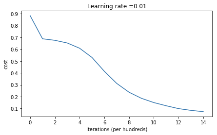
2.5.2 训练

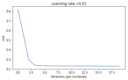
parameters = model(train_X,train_Y,initialization="he",is_polt=True)
parameters

第0次迭代，成本值为：0.8830537463419761
第1000次迭代，成本值为：0.6879825919728063
第2000次迭代，成本值为：0.6751286264523371
第3000次迭代，成本值为：0.6526117768893807
第4000次迭代，成本值为：0.6082958970572938
第5000次迭代，成本值为：0.5304944491717495
第6000次迭代，成本值为：0.4138645817071795
第7000次迭代，成本值为：0.31178034648444414
第8000次迭代，成本值为：0.2369621533032257
第9000次迭代，成本值为：0.18597287209206845
第10000次迭代，成本值为：0.1501555628037181
第11000次迭代，成本值为：0.12325079292273548
第12000次迭代，成本值为：0.09917746546525937
第13000次迭代，成本值为：0.08457055954024273
第14000次迭代，成本值为：0.07357895962677366

在这里插入图片描述

{'W1': array([[ 2.26930788,  1.0373042 ],
        [ 0.66677708, -2.30154225],
        [-0.29367404, -0.47621019],
        [-0.56431372, -1.28550611],
        [-0.0833954 , -0.37767036],
        [-2.61667211,  0.58998578],
        [ 1.17205304,  2.13928934],
        [ 0.29920508, -0.71480482],
        [-0.76036578, -1.72129222],
        [ 1.6007726 , -1.84027265]]),
 'W2': array([[-0.53142441, -0.09196943,  0.66462575,  0.10586273, -0.45785063,
         -0.32575065,  0.26529788, -0.07193113, -0.34383407, -0.10287287],
        [ 0.38133683,  0.77564511, -0.62439683, -0.41578462, -0.35406464,
         -0.99607919, -0.29606634,  0.23084402,  0.42275344, -0.25953776],
        [-0.72595532,  0.28920205, -0.15932913, -0.77955637, -0.26682983,
         -0.26322741, -0.39081204,  0.01328842, -1.00545144, -0.11974675],
        [ 0.12787355,  0.3388063 ,  0.48200186,  0.48460282,  0.65301573,
         -0.52408346, -0.02795833, -0.84266062, -0.31640932, -0.88706719],
        [ 1.80657865,  1.69960454,  0.32553862,  1.54847526, -0.17913703,
          2.2019285 ,  1.6481392 , -1.96449025,  1.06244244,  2.12191174]]),
 'W3': array([[-0.64865924,  0.99662957, -0.09771871,  0.9989112 , -5.3370528 ]]),
 'b1': array([[-0.23394446],
        [-0.25110623],
        [-0.23443956],
        [-0.52496578],
        [ 0.03367351],
        [ 0.09107832],
        [-0.47678099],
        [ 1.74920979],
        [-0.43799719],
        [-0.31092435]]),
 'b2': array([[-0.04860647],
        [ 1.03523628],
        [ 0.        ],
        [-0.17145413],
        [-2.23070032]]),
 'b3': array([[2.8409238]])}

2.5.3 预测

print ("训练集:")
predictions_train = init_utils.predict(train_X, train_Y, parameters)
print ("测试集:")
predictions_test = init_utils.predict(test_X, test_Y, parameters)

训练集:
Accuracy: 0.9933333333333333
测试集:
Accuracy: 0.96

卧槽相当牛逼了，比上面的精度高了很多！

2.6 总结

不同的初始化方法可能导致性能最终不同
随机初始化有助于打破对称，使得不同隐藏层的单元可以学习到不同的参数。
初始化时，初始值不宜过大。
He初始化搭配ReLU激活函数常常可以得到不错的效果。

3 正则化

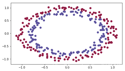
3.1 数据

import scipy.io as sio

def load_2D_dataset(is_plot=True):
    data = sio.loadmat('datasets/data.mat')
    train_X = data['X'].T
    train_Y = data['y'].T
    test_X = data['Xval'].T
    test_Y = data['yval'].T
    if is_plot:
        plt.scatter(train_X[0, :], train_X[1, :], c=np.squeeze(train_Y), s=40, cmap=plt.cm.Spectral);
    
    return train_X, train_Y, test_X, test_Y

train_X, train_Y, test_X, test_Y = load_2D_dataset(is_plot=True)

在这里插入图片描述

3.2 代码

由于引入正则化，损失函数的公式增加了一项，所以计算cost以及反向传播cost的代码需要变化

def compute_cost_with_regularization(A3,Y,parameters,lambd):
    """
    实现公式2的L2正则化计算成本

    参数：
        A3 - 正向传播的输出结果，维度为（输出节点数量，训练/测试的数量）
        Y - 标签向量，与数据一一对应，维度为(输出节点数量，训练/测试的数量)
        parameters - 包含模型学习后的参数的字典
    返回：
        cost - 使用公式2计算出来的正则化损失的值

    """
    m = Y.shape[1]
    W1 = parameters["W1"]
    W2 = parameters["W2"]
    W3 = parameters["W3"]

    cross_entropy_cost = reg_utils.compute_cost(A3,Y)

    L2_regularization_cost = lambd * (np.sum(np.square(W1)) + np.sum(np.square(W2))  + np.sum(np.square(W3))) / (2 * m)

    cost = cross_entropy_cost + L2_regularization_cost

    return cost

#当然，因为改变了成本函数，我们也必须改变向后传播的函数， 所有的梯度都必须根据这个新的成本值来计算。

def backward_propagation_with_regularization(X, Y, cache, lambd):
    """
    实现我们添加了L2正则化的模型的后向传播。

    参数：
        X - 输入数据集，维度为（输入节点数量，数据集里面的数量）
        Y - 标签，维度为（输出节点数量，数据集里面的数量）
        cache - 来自forward_propagation（）的cache输出
        lambda - regularization超参数，实数

    返回：
        gradients - 一个包含了每个参数、激活值和预激活值变量的梯度的字典
    """

    m = X.shape[1]

    (Z1, A1, W1, b1, Z2, A2, W2, b2, Z3, A3, W3, b3) = cache

    dZ3 = A3 - Y

    dW3 = (1 / m) * np.dot(dZ3,A2.T) + ((lambd * W3) / m )
    db3 = (1 / m) * np.sum(dZ3,axis=1,keepdims=True)

    dA2 = np.dot(W3.T,dZ3)
    dZ2 = np.multiply(dA2,np.int64(A2 > 0))
    dW2 = (1 / m) * np.dot(dZ2,A1.T) + ((lambd * W2) / m)
    db2 = (1 / m) * np.sum(dZ2,axis=1,keepdims=True)

    dA1 = np.dot(W2.T,dZ2)
    dZ1 = np.multiply(dA1,np.int64(A1 > 0))
    dW1 = (1 / m) * np.dot(dZ1,X.T) + ((lambd * W1) / m)
    db1 = (1 / m) * np.sum(dZ1,axis=1,keepdims=True)

    gradients = {"dZ3": dZ3, "dW3": dW3, "db3": db3, "dA2": dA2,
                 "dZ2": dZ2, "dW2": dW2, "db2": db2, "dA1": dA1, 
                 "dZ1": dZ1, "dW1": dW1, "db1": db1}

    return gradients

def model(X,Y,learning_rate=0.01,num_iterations=15000, lambd=0, print_cost=True,initialization="he",is_polt=True):
    """
    实现一个三层的神经网络：LINEAR ->RELU -> LINEAR -> RELU -> LINEAR -> SIGMOID

    参数：
        X - 输入的数据，维度为(2, 要训练/测试的数量)
        Y - 标签，【0 | 1】，维度为(1，对应的是输入的数据的标签)
        learning_rate - 学习速率
        num_iterations - 迭代的次数
        print_cost - 是否打印成本值，每迭代1000次打印一次
        initialization - 字符串类型，初始化的类型【"zeros" | "random" | "he"】
        is_polt - 是否绘制梯度下降的曲线图
        lambd - 正则化参数
    返回
        parameters - 学习后的参数
    """
    grads = {}
    costs = []
    m = X.shape[1]
    layers_dims = [X.shape[0],10,5,1]

    #选择初始化参数的类型
    if initialization == "zeros":
        parameters = initialize_parameters_zeros(layers_dims)
    elif initialization == "random":
        parameters = initialize_parameters_random(layers_dims)
    elif initialization == "he":
        parameters = initialize_parameters_he(layers_dims)
    else : 
        print("错误的初始化参数！程序退出")
        exit

    #开始学习
    for i in range(0,num_iterations):
        #前向传播
        a3 , cache = init_utils.forward_propagation(X,parameters)

        #计算成本        
        cost = init_utils.compute_loss(a3,Y)

        #反向传播
        grads = init_utils.backward_propagation(X,Y,cache)

        #更新参数
        parameters = init_utils.update_parameters(parameters,grads,learning_rate)

        #记录成本
        if i % 1000 == 0:
            costs.append(cost)
            #打印成本
            if print_cost:
                print("第" + str(i) + "次迭代，成本值为：" + str(cost))


    #学习完毕，绘制成本曲线
    if is_polt:
        plt.plot(costs)
        plt.ylabel('cost')
        plt.xlabel('iterations (per hundreds)')
        plt.title("Learning rate =" + str(learning_rate))
        plt.show()

    #返回学习完毕后的参数
    return parameters

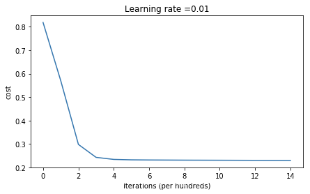
3.3 训练+预测

parameters = model(train_X, train_Y, lambd=0.7,is_polt=True)
print("使用正则化，训练集:")
predictions_train = reg_utils.predict(train_X, train_Y, parameters)
print("使用正则化，测试集:")
predictions_test = reg_utils.predict(test_X, test_Y, parameters)

第0次迭代，成本值为：0.8182760536998407
第1000次迭代，成本值为：0.5702210539472338
第2000次迭代，成本值为：0.29835042886732865
第3000次迭代，成本值为：0.2432883931921556
第4000次迭代，成本值为：0.2344959083427152
第5000次迭代，成本值为：0.23264777653673396
第6000次迭代，成本值为：0.23204990707849468
第7000次迭代，成本值为：0.23171085396182836
第8000次迭代，成本值为：0.23137427703179395
第9000次迭代，成本值为：0.23116201993351987
第10000次迭代，成本值为：0.23096258775937067
第11000次迭代，成本值为：0.2307495523856153
第12000次迭代，成本值为：0.23054651748350388
第13000次迭代，成本值为：0.23032100457597718
第14000次迭代，成本值为：0.2300877112237079

在这里插入图片描述

使用正则化，训练集:
Accuracy: 0.919431279620853
使用正则化，测试集:
Accuracy: 0.915

正则化之后虽然准确率没有上面未正则化的高，但应该能有效避免过拟合的情况！

parameters = model(train_X, train_Y,is_polt=True,lambd=0.7,num_iterations=20000)
print("使用正则化，训练集:")
predictions_train = reg_utils.predict(train_X, train_Y, parameters)
print("使用正则化，测试集:")
predictions_test = reg_utils.predict(test_X, test_Y, parameters)

第0次迭代，成本值为：0.8182760536998407
第1000次迭代，成本值为：0.5702210539472338
第2000次迭代，成本值为：0.29835042886732865
第3000次迭代，成本值为：0.2432883931921556
第4000次迭代，成本值为：0.2344959083427152
第5000次迭代，成本值为：0.23264777653673396
第6000次迭代，成本值为：0.23204990707849468
第7000次迭代，成本值为：0.23171085396182836
第8000次迭代，成本值为：0.23137427703179395
第9000次迭代，成本值为：0.23116201993351987
第10000次迭代，成本值为：0.23096258775937067
第11000次迭代，成本值为：0.2307495523856153
第12000次迭代，成本值为：0.23054651748350388
第13000次迭代，成本值为：0.23032100457597718
第14000次迭代，成本值为：0.2300877112237079
第15000次迭代，成本值为：0.22992655305094892
第16000次迭代，成本值为：0.2297797758224707
第17000次迭代，成本值为：0.22960314250832073
第18000次迭代，成本值为：0.22929240624776243
第19000次迭代，成本值为：0.2288307047561804

在这里插入图片描述

使用正则化，训练集:
Accuracy: 0.9241706161137441
使用正则化，测试集:
Accuracy: 0.915

4 dropout

需要修改代码的部分为前向传播和反向传播的过程，因为有些神经元失活了

4.1 代码

4.1.1前向

def forward_propagation_with_dropout(X,parameters,keep_prob=0.5):
    """
    实现具有随机舍弃节点的前向传播。
    LINEAR -> RELU + DROPOUT -> LINEAR -> RELU + DROPOUT -> LINEAR -> SIGMOID.

    参数：
        X  - 输入数据集，维度为（2，示例数）
        parameters - 包含参数“W1”，“b1”，“W2”，“b2”，“W3”，“b3”的python字典：
            W1  - 权重矩阵，维度为（20,2）
            b1  - 偏向量，维度为（20,1）
            W2  - 权重矩阵，维度为（3,20）
            b2  - 偏向量，维度为（3,1）
            W3  - 权重矩阵，维度为（1,3）
            b3  - 偏向量，维度为（1,1）
        keep_prob  - 随机删除的概率，实数
    返回：
        A3  - 最后的激活值，维度为（1,1），正向传播的输出
        cache - 存储了一些用于计算反向传播的数值的元组
    """
    np.random.seed(1)

    W1 = parameters["W1"]
    b1 = parameters["b1"]
    W2 = parameters["W2"]
    b2 = parameters["b2"]
    W3 = parameters["W3"]
    b3 = parameters["b3"]

    #LINEAR -> RELU -> LINEAR -> RELU -> LINEAR -> SIGMOID
    Z1 = np.dot(W1,X) + b1
    A1 = reg_utils.relu(Z1) # 激活后的值 但要失活一部分 所以有下面的代码

    #下面的步骤1-4对应于上述的步骤1-4。
    D1 = np.random.rand(A1.shape[0],A1.shape[1])    #步骤1：初始化矩阵D1 = np.random.rand(..., ...)
    D1 = D1 < keep_prob                             #步骤2：将D1的值转换为0或1（使用keep_prob作为阈值）
    A1 = A1 * D1                                    #步骤3：舍弃A1的一些节点（将它的值变为0或False）
    A1 = A1 / keep_prob                             #步骤4：缩放未舍弃的节点(不为0)的值
    """
    #不理解的同学运行一下下面代码就知道了。
    import numpy as np
    np.random.seed(1)
    A1 = np.random.randn(1,3)

    D1 = np.random.rand(A1.shape[0],A1.shape[1])
    keep_prob=0.5
    D1 = D1 < keep_prob
    print(D1)

    A1 = 0.01
    A1 = A1 * D1
    A1 = A1 / keep_prob
    print(A1)
    """

    Z2 = np.dot(W2,A1) + b2
    A2 = reg_utils.relu(Z2)

    #下面的步骤1-4对应于上述的步骤1-4。
    D2 = np.random.rand(A2.shape[0],A2.shape[1])    #步骤1：初始化矩阵D2 = np.random.rand(..., ...)
    D2 = D2 < keep_prob                             #步骤2：将D2的值转换为0或1（使用keep_prob作为阈值）
    A2 = A2 * D2                                    #步骤3：舍弃A1的一些节点（将它的值变为0或False）
    A2 = A2 / keep_prob                             #步骤4：缩放未舍弃的节点(不为0)的值

    Z3 = np.dot(W3, A2) + b3
    A3 = reg_utils.sigmoid(Z3) # 输出就1个神经元 所以不需要失活处理

    cache = (Z1, D1, A1, W1, b1, Z2, D2, A2, W2, b2, Z3, A3, W3, b3)

    return A3, cache

4.1.2 反向

def backward_propagation_with_dropout(X,Y,cache,keep_prob):
    """
    实现我们随机删除的模型的后向传播。
    参数：
        X  - 输入数据集，维度为（2，示例数）
        Y  - 标签，维度为（输出节点数量，示例数量）
        cache - 来自forward_propagation_with_dropout（）的cache输出
        keep_prob  - 随机删除的概率，实数

    返回：
        gradients - 一个关于每个参数、激活值和预激活变量的梯度值的字典
    """
    m = X.shape[1]
    (Z1, D1, A1, W1, b1, Z2, D2, A2, W2, b2, Z3, A3, W3, b3) = cache

    dZ3 = A3 - Y
    dW3 = (1 / m) * np.dot(dZ3,A2.T)
    db3 = 1. / m * np.sum(dZ3, axis=1, keepdims=True)
    dA2 = np.dot(W3.T, dZ3)

    dA2 = dA2 * D2          # 步骤1：使用正向传播期间相同的节点，舍弃那些关闭的节点（因为任何数乘以0或者False都为0或者False）
    dA2 = dA2 / keep_prob   # 步骤2：缩放未舍弃的节点(不为0)的值

    dZ2 = np.multiply(dA2, np.int64(A2 > 0))
    dW2 = 1. / m * np.dot(dZ2, A1.T)
    db2 = 1. / m * np.sum(dZ2, axis=1, keepdims=True)

    dA1 = np.dot(W2.T, dZ2)

    dA1 = dA1 * D1          # 步骤1：使用正向传播期间相同的节点，舍弃那些关闭的节点（因为任何数乘以0或者False都为0或者False）
    dA1 = dA1 / keep_prob   # 步骤2：缩放未舍弃的节点(不为0)的值

    dZ1 = np.multiply(dA1, np.int64(A1 > 0))
    dW1 = 1. / m * np.dot(dZ1, X.T)
    db1 = 1. / m * np.sum(dZ1, axis=1, keepdims=True)

    gradients = {"dZ3": dZ3, "dW3": dW3, "db3": db3,"dA2": dA2,
                 "dZ2": dZ2, "dW2": dW2, "db2": db2, "dA1": dA1, 
                 "dZ1": dZ1, "dW1": dW1, "db1": db1}

    return gradients

4.1.3 主代码

def model(X,Y,learning_rate=0.01,num_iterations=15000,print_cost=True,initialization="he",is_polt=True, keep_prob=0.5):
    """
    实现一个三层的神经网络：LINEAR ->RELU -> LINEAR -> RELU -> LINEAR -> SIGMOID

    参数：
        X - 输入的数据，维度为(2, 要训练/测试的数量)
        Y - 标签，【0 | 1】，维度为(1，对应的是输入的数据的标签)
        learning_rate - 学习速率
        num_iterations - 迭代的次数
        print_cost - 是否打印成本值，每迭代1000次打印一次
        initialization - 字符串类型，初始化的类型【"zeros" | "random" | "he"】
        is_polt - 是否绘制梯度下降的曲线图
    返回
        parameters - 学习后的参数
    """
    grads = {}
    costs = []
    m = X.shape[1]
    layers_dims = [X.shape[0],10,5,1]

    #选择初始化参数的类型
    if initialization == "zeros":
        parameters = initialize_parameters_zeros(layers_dims)
    elif initialization == "random":
        parameters = initialize_parameters_random(layers_dims)
    elif initialization == "he":
        parameters = initialize_parameters_he(layers_dims)
    else : 
        print("错误的初始化参数！程序退出")
        exit

    #开始学习
    for i in range(0,num_iterations):
        #前向传播
        a3 , cache = forward_propagation_with_dropout(X,parameters,keep_prob=0.5)

        #计算成本        
        cost = init_utils.compute_loss(a3,Y)

        #反向传播
        grads = backward_propagation_with_dropout(X,Y,cache,keep_prob)

        #更新参数
        parameters = init_utils.update_parameters(parameters,grads,learning_rate)

        #记录成本
        if i % 1000 == 0:
            costs.append(cost)
            #打印成本
            if print_cost:
                print("第" + str(i) + "次迭代，成本值为：" + str(cost))


    #学习完毕，绘制成本曲线
    if is_polt:
        plt.plot(costs)
        plt.ylabel('cost')
        plt.xlabel('iterations (per hundreds)')
        plt.title("Learning rate =" + str(learning_rate))
        plt.show()

    #返回学习完毕后的参数
    return parameters

4.2 训练+预测

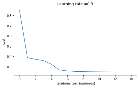
parameters = model(train_X, train_Y, keep_prob=0.86, learning_rate=0.3,is_polt=True)

print("使用随机删除节点，训练集:")
predictions_train = reg_utils.predict(train_X, train_Y, parameters)
print("使用随机删除节点，测试集:")
reg_utils.predictions_test = reg_utils.predict(test_X, test_Y, parameters)

第0次迭代，成本值为：0.8507860147818928
第1000次迭代，成本值为：0.3873714180471037
第2000次迭代，成本值为：0.3720394089743302
第3000次迭代，成本值为：0.35982370299095773
第4000次迭代，成本值为：0.3239536446466947


/Users/apple/Desktop/深度学习/课程2-week1/init_utils.py:50: RuntimeWarning: divide by zero encountered in log
  logprobs = np.multiply(-np.log(a3),Y) + np.multiply(-np.log(1 - a3), 1 - Y)
/Users/apple/Desktop/深度学习/课程2-week1/init_utils.py:50: RuntimeWarning: invalid value encountered in multiply
  logprobs = np.multiply(-np.log(a3),Y) + np.multiply(-np.log(1 - a3), 1 - Y)


第5000次迭代，成本值为：0.26833101413187094
第6000次迭代，成本值为：0.2590069112583366
第7000次迭代，成本值为：0.2542389928282903
第8000次迭代，成本值为：0.25224163263185556
第9000次迭代，成本值为：0.25109259309986964
第10000次迭代，成本值为：0.2503088273978559
第11000次迭代，成本值为：0.2497141227182644
第12000次迭代，成本值为：0.2494909360725536
第13000次迭代，成本值为：0.24923710314189443
第14000次迭代，成本值为：0.2489525908753509

在这里插入图片描述

使用随机删除节点，训练集:
Accuracy: 0.9241706161137441
使用随机删除节点，测试集:
Accuracy: 0.91

用dropout运行模型（keep_prob = 0.86）跑一波。这意味着在每次迭代中，程序都可以24％的概率关闭第1层和第2层的每个神经元。

5 梯度校验

本质上做的事情是：看dw db和直接根据导数公式近似的值是否差异很大如果很大可能出现了bug

5.1 一维情形

5.1.1 前向传播

def forward_propagation(x,theta):
    """

    实现图中呈现的线性前向传播（计算J）（J（theta）= theta * x）

    参数：
    x  - 一个实值输入
    theta  - 参数，也是一个实数

    返回：
    J  - 函数J的值，用公式J（theta）= theta * x计算
    """
    J = np.dot(theta,x)

    return J

5.1.2 反向传播

def backward_propagation(x,theta):
    """
    计算J相对于θ的导数。

    参数：
        x  - 一个实值输入
        theta  - 参数，也是一个实数

    返回：
        dtheta  - 相对于θ的成本梯度
    """
    dtheta = x

    return dtheta

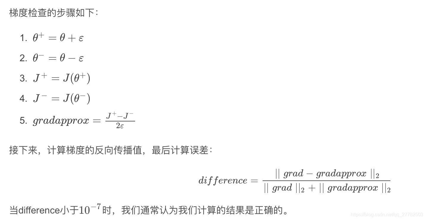
5.1.3 梯度校验

原理

def gradient_check(x,theta,epsilon=1e-7):
    """

    实现图中的反向传播。

    参数：
        x  - 一个实值输入
        theta  - 参数，也是一个实数
        epsilon  - 使用公式（3）计算输入的微小偏移以计算近似梯度

    返回：
        近似梯度和后向传播梯度之间的差异
    """

    #使用公式（3）的左侧计算gradapprox。
    thetaplus = theta + epsilon                               # Step 1
    thetaminus = theta - epsilon                              # Step 2
    J_plus = forward_propagation(x, thetaplus)                # Step 3
    J_minus = forward_propagation(x, thetaminus)              # Step 4
    gradapprox = (J_plus - J_minus) / (2 * epsilon)           # Step 5


    #检查gradapprox是否足够接近backward_propagation（）的输出
    grad = backward_propagation(x, theta)

    numerator = np.linalg.norm(grad - gradapprox)                      # Step 1' 计算L2范数
    denominator = np.linalg.norm(grad) + np.linalg.norm(gradapprox)    # Step 2'
    difference = numerator / denominator                               # Step 3'

    if difference < 1e-7:
        print("梯度检查：梯度正常!")
    else:
        print("梯度检查：梯度超出阈值!")

    return difference

5.1.4 测试

#测试gradient_check
print("-----------------测试gradient_check-----------------")
x, theta = 2, 4
difference = gradient_check(x, theta)
print("difference = " + str(difference))

-----------------测试gradient_check-----------------
梯度检查：梯度正常!
difference = 2.919335883291695e-10

5.2 高维情形

5.2.1 前向传播+反向传播

def forward_propagation_n(X,Y,parameters):
    """
    实现图中的前向传播（并计算成本）。

    参数：
        X - 训练集为m个例子
        Y -  m个示例的标签
        parameters - 包含参数“W1”，“b1”，“W2”，“b2”，“W3”，“b3”的python字典：
            W1  - 权重矩阵，维度为（5,4）
            b1  - 偏向量，维度为（5,1）
            W2  - 权重矩阵，维度为（3,5）
            b2  - 偏向量，维度为（3,1）
            W3  - 权重矩阵，维度为（1,3）
            b3  - 偏向量，维度为（1,1）

    返回：
        cost - 成本函数（logistic）
    """
    m = X.shape[1]
    W1 = parameters["W1"]
    b1 = parameters["b1"]
    W2 = parameters["W2"]
    b2 = parameters["b2"]
    W3 = parameters["W3"]
    b3 = parameters["b3"]

    # LINEAR -> RELU -> LINEAR -> RELU -> LINEAR -> SIGMOID
    Z1 = np.dot(W1,X) + b1
    A1 = gc_utils.relu(Z1)

    Z2 = np.dot(W2,A1) + b2
    A2 = gc_utils.relu(Z2)

    Z3 = np.dot(W3,A2) + b3
    A3 = gc_utils.sigmoid(Z3)

    #计算成本
    logprobs = np.multiply(-np.log(A3), Y) + np.multiply(-np.log(1 - A3), 1 - Y)
    cost = (1 / m) * np.sum(logprobs)

    cache = (Z1, A1, W1, b1, Z2, A2, W2, b2, Z3, A3, W3, b3)

    return cost, cache

def backward_propagation_n(X,Y,cache):
    """
    实现图中所示的反向传播。

    参数：
        X - 输入数据点（输入节点数量，1）
        Y - 标签
        cache - 来自forward_propagation_n（）的cache输出

    返回：
        gradients - 一个字典，其中包含与每个参数、激活和激活前变量相关的成本梯度。
    """
    m = X.shape[1]
    (Z1, A1, W1, b1, Z2, A2, W2, b2, Z3, A3, W3, b3) = cache

    dZ3 = A3 - Y
    dW3 = (1. / m) * np.dot(dZ3,A2.T)
    dW3 = 1. / m * np.dot(dZ3, A2.T)
    db3 = 1. / m * np.sum(dZ3, axis=1, keepdims=True)

    dA2 = np.dot(W3.T, dZ3)
    dZ2 = np.multiply(dA2, np.int64(A2 > 0))
    #dW2 = 1. / m * np.dot(dZ2, A1.T) * 2  # Should not multiply by 2
    dW2 = 1. / m * np.dot(dZ2, A1.T)
    db2 = 1. / m * np.sum(dZ2, axis=1, keepdims=True)

    dA1 = np.dot(W2.T, dZ2)
    dZ1 = np.multiply(dA1, np.int64(A1 > 0))
    dW1 = 1. / m * np.dot(dZ1, X.T)
    #db1 = 4. / m * np.sum(dZ1, axis=1, keepdims=True) # Should not multiply by 4
    db1 = 1. / m * np.sum(dZ1, axis=1, keepdims=True)

    gradients = {"dZ3": dZ3, "dW3": dW3, "db3": db3,
                 "dA2": dA2, "dZ2": dZ2, "dW2": dW2, "db2": db2,
                 "dA1": dA1, "dZ1": dZ1, "dW1": dW1, "db1": db1}

    return gradients

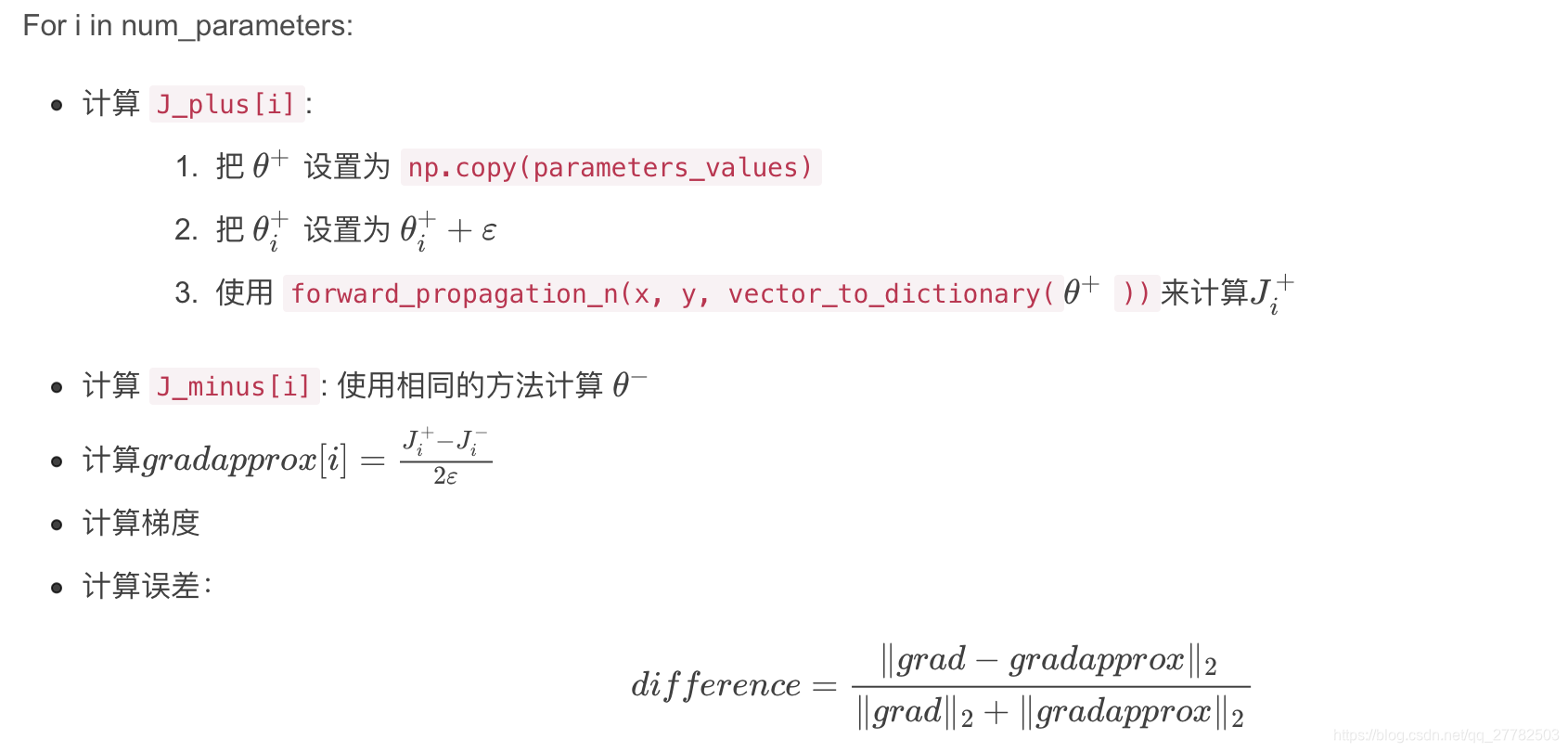
5.2.2 梯度校验

原理

def gradient_check_n(parameters,gradients,X,Y,epsilon=1e-7):
    """
    检查backward_propagation_n是否正确计算forward_propagation_n输出的成本梯度

    参数：
        parameters - 包含参数“W1”，“b1”，“W2”，“b2”，“W3”，“b3”的python字典：
        grad_output_propagation_n的输出包含与参数相关的成本梯度。
        x  - 输入数据点，维度为（输入节点数量，1）
        y  - 标签
        epsilon  - 计算输入的微小偏移以计算近似梯度

    返回：
        difference - 近似梯度和后向传播梯度之间的差异
    """
    #初始化参数
    parameters_values , keys = gc_utils.dictionary_to_vector(parameters) #keys用不到
    grad = gc_utils.gradients_to_vector(gradients)
    num_parameters = parameters_values.shape[0]
    J_plus = np.zeros((num_parameters,1))
    J_minus = np.zeros((num_parameters,1))
    gradapprox = np.zeros((num_parameters,1))

    #计算gradapprox
    for i in range(num_parameters):
        #计算J_plus [i]。输入：“parameters_values，epsilon”。输出=“J_plus [i]”
        thetaplus = np.copy(parameters_values)                                                  # Step 1
        thetaplus[i][0] = thetaplus[i][0] + epsilon                                             # Step 2
        J_plus[i], cache = forward_propagation_n(X,Y,gc_utils.vector_to_dictionary(thetaplus))  # Step 3 ，cache用不到

        #计算J_minus [i]。输入：“parameters_values，epsilon”。输出=“J_minus [i]”。
        thetaminus = np.copy(parameters_values)                                                 # Step 1
        thetaminus[i][0] = thetaminus[i][0] - epsilon                                           # Step 2        
        J_minus[i], cache = forward_propagation_n(X,Y,gc_utils.vector_to_dictionary(thetaminus))# Step 3 ，cache用不到

        #计算gradapprox[i]
        gradapprox[i] = (J_plus[i] - J_minus[i]) / (2 * epsilon)

    #通过计算差异比较gradapprox和后向传播梯度。
    numerator = np.linalg.norm(grad - gradapprox)                                     # Step 1'
    denominator = np.linalg.norm(grad) + np.linalg.norm(gradapprox)                   # Step 2'
    difference = numerator / denominator                                              # Step 3'

    if difference < 1e-7:
        print("梯度检查：梯度正常!")
    else:
        print("梯度检查：梯度超出阈值!")

    return difference

参考

https://blog.csdn.net/u013733326/article/details/79847918#commentBox

深度学习 | 吴恩达深度学习课程2 Week1

Course2 Week1 编程作业

1 任务

2 初始化参数

2.1 数据

2.2 神经网络模型

2.3 初始化为零

2.3.1 代码

2.3.2 训练

2.3.3 预测

2.4 随机初始化

2.4.1 代码

2.4.2 训练

2.4.3 预测

2.5 抑梯度异常初始化

2.5.1 代码

2.5.2 训练

2.5.3 预测

2.6 总结

3 正则化

3.1 数据

3.2 代码

3.3 训练+预测

4 dropout

4.1 代码

4.1.1前向

4.1.2 反向

4.1.3 主代码

4.2 训练+预测

5 梯度校验

5.1 一维情形

5.1.1 前向传播

5.1.2 反向传播

5.1.3 梯度校验

5.1.4 测试

5.2 高维情形

5.2.1 前向传播+反向传播

5.2.2 梯度校验

参考

猜你喜欢