P0 前言
- 第二门课 : Improving Deep Neural Networks: Hyperparameter turing,Regularization and Optimization (改善深层神经网络:超参数调试、正则化以及优化)
- 第一周 : Practical aspects of Deep Learning (深度学习的实践层面)
- 主要知识点 : (Train/Dev/Test sets)训练测试集划分、(Bias / Variance)偏差和方差、(Regulation)正则化、Dropout、(Normalizing inputs)输入归一化、(Vanishing / Exploding gradients)梯度消失与梯度爆炸、(Weight Initialization for Deep NN)权重初始化、(Gradient checking)梯度检验等
视频地址 : https://mooc.study.163.com/course/2001281003
笔记地址:https://blog.csdn.net/zongza/article/details/83020267
数据集,源码,作业的本地版网页缓存下载:链接: https://pan.baidu.com/s/1FCxBfVGHDprAYZdZJXNGZg 提取码: f6xn
P1 作业
第一部分:初始化
该部分作业的原始网页:链接: https://pan.baidu.com/s/1_Inl5XQmjbxuI6Z8wia5Rw 提取码: yg8c
一个好的初始化可以:
- 加速梯度下降的收敛过程
- 增加梯度下降收敛到一个较低训练误差(泛化误差)的几率
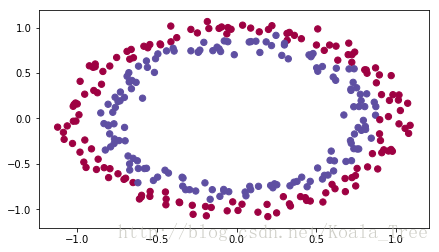
运行下面单元加载工具包和需要你进行分类的平面数据集。
import numpy as np
import matplotlib.pyplot as plt
import sklearn
import sklearn.datasets
from init_utils import sigmoid, relu, compute_loss, forward_propagation, backward_propagation
from init_utils import update_parameters, predict, load_dataset, plot_decision_boundary, predict_dec

%matplotlib inline
plt.rcParams['figure.figsize'] = (7.0, 4.0) # set default size of plots
plt.rcParams['image.interpolation'] = 'nearest'
plt.rcParams['image.cmap'] = 'gray'

# load image dataset: blue/red dots in circles
train_X, train_Y, test_X, test_Y = load_dataset()
从int_utils.py所import的函数内容如下:
import numpy as np
import matplotlib.pyplot as plt
import h5py
import sklearn
import sklearn.datasets

def sigmoid(x):
    """
    Compute the sigmoid of x

    Arguments:
    x -- A scalar or numpy array of any size.

    Return:
    s -- sigmoid(x)
    """
    s = 1/(1+np.exp(-x))
    return s

def relu(x):
    """
    Compute the relu of x

    Arguments:
    x -- A scalar or numpy array of any size.

    Return:
    s -- relu(x)
    """
    s = np.maximum(0,x)

    return s

def forward_propagation(X, parameters):
    """
    Implements the forward propagation (and computes the loss) presented in Figure 2.

    Arguments:
    X -- input dataset, of shape (input size, number of examples)
    Y -- true "label" vector (containing 0 if cat, 1 if non-cat)
    parameters -- python dictionary containing your parameters "W1", "b1", "W2", "b2", "W3", "b3":
                    W1 -- weight matrix of shape ()
                    b1 -- bias vector of shape ()
                    W2 -- weight matrix of shape ()
                    b2 -- bias vector of shape ()
                    W3 -- weight matrix of shape ()
                    b3 -- bias vector of shape ()

    Returns:
    loss -- the loss function (vanilla logistic loss)
    """

    # retrieve parameters
    W1 = parameters["W1"]
    b1 = parameters["b1"]
    W2 = parameters["W2"]
    b2 = parameters["b2"]
    W3 = parameters["W3"]
    b3 = parameters["b3"]

    # LINEAR -> RELU -> LINEAR -> RELU -> LINEAR -> SIGMOID
    z1 = np.dot(W1, X) + b1
    a1 = relu(z1)
    z2 = np.dot(W2, a1) + b2
    a2 = relu(z2)
    z3 = np.dot(W3, a2) + b3
    a3 = sigmoid(z3)

    cache = (z1, a1, W1, b1, z2, a2, W2, b2, z3, a3, W3, b3)

    return a3, cache

def backward_propagation(X, Y, cache):
    """
    Implement the backward propagation presented in figure 2.

    Arguments:
    X -- input dataset, of shape (input size, number of examples)
    Y -- true "label" vector (containing 0 if cat, 1 if non-cat)
    cache -- cache output from forward_propagation()

    Returns:
    gradients -- A dictionary with the gradients with respect to each parameter, activation and pre-activation variables
    """
    m = X.shape[1]
    (z1, a1, W1, b1, z2, a2, W2, b2, z3, a3, W3, b3) = cache

    dz3 = 1./m * (a3 - Y)
    dW3 = np.dot(dz3, a2.T)
    db3 = np.sum(dz3, axis=1, keepdims = True)

    da2 = np.dot(W3.T, dz3)
    dz2 = np.multiply(da2, np.int64(a2 > 0))
    dW2 = np.dot(dz2, a1.T)
    db2 = np.sum(dz2, axis=1, keepdims = True)

    da1 = np.dot(W2.T, dz2)
    dz1 = np.multiply(da1, np.int64(a1 > 0))
    dW1 = np.dot(dz1, X.T)
    db1 = np.sum(dz1, axis=1, keepdims = True)

    gradients = {"dz3": dz3, "dW3": dW3, "db3": db3,
                 "da2": da2, "dz2": dz2, "dW2": dW2, "db2": db2,
                 "da1": da1, "dz1": dz1, "dW1": dW1, "db1": db1}

    return gradients

def update_parameters(parameters, grads, learning_rate):
    """
    Update parameters using gradient descent

    Arguments:
    parameters -- python dictionary containing your parameters
    grads -- python dictionary containing your gradients, output of n_model_backward

    Returns:
    parameters -- python dictionary containing your updated parameters
                  parameters['W' + str(i)] = ...
                  parameters['b' + str(i)] = ...
    """

    L = len(parameters) // 2 # number of layers in the neural networks

    # Update rule for each parameter
    for k in range(L):
        parameters["W" + str(k+1)] = parameters["W" + str(k+1)] - learning_rate * grads["dW" + str(k+1)]
        parameters["b" + str(k+1)] = parameters["b" + str(k+1)] - learning_rate * grads["db" + str(k+1)]

    return parameters

def compute_loss(a3, Y):

    """
    Implement the loss function

    Arguments:
    a3 -- post-activation, output of forward propagation
    Y -- "true" labels vector, same shape as a3

    Returns:
    loss - value of the loss function
    """

    m = Y.shape[1]
    logprobs = np.multiply(-np.log(a3),Y) + np.multiply(-np.log(1 - a3), 1 - Y)
    loss = 1./m * np.nansum(logprobs)

    return loss

def load_cat_dataset():
    train_dataset = h5py.File('datasets/train_catvnoncat.h5', "r")
    train_set_x_orig = np.array(train_dataset["train_set_x"][:]) # your train set features
    train_set_y_orig = np.array(train_dataset["train_set_y"][:]) # your train set labels

    test_dataset = h5py.File('datasets/test_catvnoncat.h5', "r")
    test_set_x_orig = np.array(test_dataset["test_set_x"][:]) # your test set features
    test_set_y_orig = np.array(test_dataset["test_set_y"][:]) # your test set labels

    classes = np.array(test_dataset["list_classes"][:]) # the list of classes

    train_set_y = train_set_y_orig.reshape((1, train_set_y_orig.shape[0]))
    test_set_y = test_set_y_orig.reshape((1, test_set_y_orig.shape[0]))

    train_set_x_orig = train_set_x_orig.reshape(train_set_x_orig.shape[0], -1).T
    test_set_x_orig = test_set_x_orig.reshape(test_set_x_orig.shape[0], -1).T

    train_set_x = train_set_x_orig/255
    test_set_x = test_set_x_orig/255

    return train_set_x, train_set_y, test_set_x, test_set_y, classes


def predict(X, y, parameters):
    """
    This function is used to predict the results of a  n-layer neural network.

    Arguments:
    X -- data set of examples you would like to label
    parameters -- parameters of the trained model

    Returns:
    p -- predictions for the given dataset X
    """

    m = X.shape[1]
    p = np.zeros((1,m), dtype = np.int)

    # Forward propagation
    a3, caches = forward_propagation(X, parameters)

    # convert probas to 0/1 predictions
    for i in range(0, a3.shape[1]):
        if a3[0,i] > 0.5:
            p[0,i] = 1
        else:
            p[0,i] = 0

    # print results
    print("Accuracy: "  + str(np.mean((p[0,:] == y[0,:]))))

    return p

def plot_decision_boundary(model, X, y):
    # Set min and max values and give it some padding
    x_min, x_max = X[0, :].min() - 1, X[0, :].max() + 1
    y_min, y_max = X[1, :].min() - 1, X[1, :].max() + 1
    h = 0.01
    # Generate a grid of points with distance h between them
    xx, yy = np.meshgrid(np.arange(x_min, x_max, h), np.arange(y_min, y_max, h))
    # Predict the function value for the whole grid
    Z = model(np.c_[xx.ravel(), yy.ravel()])
    Z = Z.reshape(xx.shape)
    # Plot the contour and training examples
    plt.contourf(xx, yy, Z, cmap=plt.cm.Spectral)
    plt.ylabel('x2')
    plt.xlabel('x1')
    plt.scatter(X[0, :], X[1, :], c=y, cmap=plt.cm.Spectral)
    plt.show()

def predict_dec(parameters, X):
    """
    Used for plotting decision boundary.

    Arguments:
    parameters -- python dictionary containing your parameters
    X -- input data of size (m, K)

    Returns
    predictions -- vector of predictions of our model (red: 0 / blue: 1)
    """

    # Predict using forward propagation and a classification threshold of 0.5
    a3, cache = forward_propagation(X, parameters)
    predictions = (a3>0.5)
    return predictions

def load_dataset():
    np.random.seed(1)
    train_X, train_Y = sklearn.datasets.make_circles(n_samples=300, noise=.05)
    np.random.seed(2)
    test_X, test_Y = sklearn.datasets.make_circles(n_samples=100, noise=.05)
    # Visualize the data
    plt.scatter(train_X[:, 0], train_X[:, 1], c=train_Y, s=40, cmap=plt.cm.Spectral);
    train_X = train_X.T
    train_Y = train_Y.reshape((1, train_Y.shape[0]))
    test_X = test_X.T
    test_Y = test_Y.reshape((1, test_Y.shape[0]))
    return train_X, train_Y, test_X, test_Y
1- 神经网络模型
你将会使用一个三层的神经网络(已经为你实现好了)这是三种你需要进行测试的初始化方法:
- Zeros initialization :在下面的model函数的输入参数中设置 initialization = "zeros"
- Random initialization :设置initialization = "random",这会使得权重矩阵W的初始值是一个较大的随机值
- He initialization :设置initialization = "he",这将权重初始化为根据He的论文缩放(scaled)的随机值
说明:请快速阅读以下代码并运行它,下一节你将实现model()所调用的这三种初始化方式
def model(X, Y, learning_rate = 0.01, num_iterations = 15000, print_cost = True, initialization = "he"):
    """
    Implements a three-layer neural network: LINEAR->RELU->LINEAR->RELU->LINEAR->SIGMOID.

    Arguments:
    X -- input data, of shape (2, number of examples)
    Y -- true "label" vector (containing 0 for red dots; 1 for blue dots), of shape (1, number of examples)
    learning_rate -- learning rate for gradient descent
    num_iterations -- number of iterations to run gradient descent
    print_cost -- if True, print the cost every 1000 iterations
    initialization -- flag to choose which initialization to use ("zeros","random" or "he")

    Returns:
    parameters -- parameters learnt by the model
    """

    grads = {}
    costs = [] # to keep track of the loss
    m = X.shape[1] # number of examples
    layers_dims = [X.shape[0], 10, 5, 1]

    # Initialize parameters dictionary.
    if initialization == "zeros":
        parameters = initialize_parameters_zeros(layers_dims)
    elif initialization == "random":
        parameters = initialize_parameters_random(layers_dims)
    elif initialization == "he":
        parameters = initialize_parameters_he(layers_dims)

    # Loop (gradient descent)

    for i in range(0, num_iterations):

        # Forward propagation: LINEAR -> RELU -> LINEAR -> RELU -> LINEAR -> SIGMOID.
        a3, cache = forward_propagation(X, parameters)

        # Loss
        cost = compute_loss(a3, Y)

        # Backward propagation.
        grads = backward_propagation(X, Y, cache)

        # Update parameters.
        parameters = update_parameters(parameters, grads, learning_rate)

        # Print the loss every 1000 iterations
        if print_cost and i % 1000 == 0:
            print("Cost after iteration {}: {}".format(i, cost))
            costs.append(cost)

    # plot the loss
    plt.plot(costs)
    plt.ylabel('cost')
    plt.xlabel('iterations (per hundreds)')
    plt.title("Learning rate =" + str(learning_rate))
    plt.show()

    return parameters
2- zero initialization
在神经网络中有两类参数需要初始化:
- 权重矩阵( the weight matrices)
- 偏置向量( the bias vectors)
练习:实现下面的零初始化函数。你将会发现这种方式并不奏效,因为他很难“打破对称”,尽管如此我们还是要先运行一下看看到底会发生什么。 请正确填充np.zeros((... , ...))
# GRADED FUNCTION: initialize_parameters_zeros

def initialize_parameters_zeros(layers_dims):
    """
    Arguments:
    layer_dims -- python array (list) containing the size of each layer.

    Returns:
    parameters -- python dictionary containing your parameters "W1", "b1", ..., "WL", "bL":
                    W1 -- weight matrix of shape (layers_dims[1], layers_dims[0])
                    b1 -- bias vector of shape (layers_dims[1], 1)
                    ...
                    WL -- weight matrix of shape (layers_dims[L], layers_dims[L-1])
                    bL -- bias vector of shape (layers_dims[L], 1)
    """

    parameters = {}
    L = len(layers_dims)            # number of layers in the network

    for l in range(1, L):
        ### START CODE HERE ### (≈ 2 lines of code)
        parameters['W' + str(l)] = np.zeros((layers_dims[l],layers_dims[l-1]))
        parameters['b' + str(l)] = np.zeros((layers_dims[l],1))
        ### END CODE HERE ###
    return parameters
parameters = initialize_parameters_zeros([3,2,1])
print("W1 = " + str(parameters["W1"]))
print("b1 = " + str(parameters["b1"]))
print("W2 = " + str(parameters["W2"]))
print("b2 = " + str(parameters["b2"]))
预计的输出值:

运行下面的代码来训练你的模型,你的参数是零初始化的并且会经过15000轮迭代更新。
parameters = model(train_X, train_Y, initialization = "zeros")
print ("On the train set:")
predictions_train = predict(train_X, train_Y, parameters)
print ("On the test set:")
predictions_test = predict(test_X, test_Y, parameters)
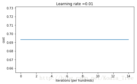

结果只能用惨烈来形容,可以看到损失(cost)实际上并没有真的减少,算法也没有比随机猜测更好。为什么?让我们看看预测和决策边界的细节)
在代码中添加下面几行:
print ("predictions_train = " + str(predictions_train))
print ("predictions_test = " + str(predictions_test))

plt.title("Model with Zeros initialization")
axes = plt.gca()
axes.set_xlim([-1.5,1.5])
axes.set_ylim([-1.5,1.5])
plot_decision_boundary(lambda x: predict_dec(parameters, x.T), train_X, np.squeeze(train_Y))
结果:


可以看到,模型将所有样本的label都预测成0。
通常,用0来初始化网络很难打破对称(break symmetry),这意味着每一层的每一个神经元学习到的都是相同的东西,你训练出来的模型和每层神经元数的模型完全一样,这种网络并不比线性分类器(logistics regression)好多少。
注意:
- 权重矩阵
应该被随机初始化从而break symmetry
是可以被初始化为0值的,(so long as)只要w是随机初始化的,symmetry就可以打破
3- Random initialization
为了打破对称,我们需要随机初始化权重,只有这样每个神经元才会从输入中学到不同的函数,在下面的练习中你会看到权重被随机初始化为一个较大的值后会发生什么。
练习:
为了初始化W为一个大值,使用 np.random.randn(..,..) * 10 (放大了十倍)对于b,使用np.zeros((.., ..)),同时我们还会使用随机种子 np.random.seed(..) 来保证每次新运行的程序获得的随机值相同
# GRADED FUNCTION: initialize_parameters_random

def initialize_parameters_random(layers_dims):
    """
    Arguments:
    layer_dims -- python array (list) containing the size of each layer.

    Returns:
    parameters -- python dictionary containing your parameters "W1", "b1", ..., "WL", "bL":
                    W1 -- weight matrix of shape (layers_dims[1], layers_dims[0])
                    b1 -- bias vector of shape (layers_dims[1], 1)
                    ...
                    WL -- weight matrix of shape (layers_dims[L], layers_dims[L-1])
                    bL -- bias vector of shape (layers_dims[L], 1)
    """

    np.random.seed(3)               # This seed makes sure your "random" numbers will be the as ours
    parameters = {}
    L = len(layers_dims)            # integer representing the number of layers

    for l in range(1, L):
        ### START CODE HERE ### (≈ 2 lines of code)
        parameters['W' + str(l)] = np.random.randn(layers_dims[l],layers_dims[l-1])*10
        parameters['b' + str(l)] = np.zeros((layers_dims[l],1))
        ### END CODE HERE ###

    return parameters
在model函数中添加:
parameters = initialize_parameters_random([3, 2, 1])
print("W1 = " + str(parameters["W1"]))
print("b1 = " + str(parameters["b1"]))
print("W2 = " + str(parameters["W2"]))
print("b2 = " + str(parameters["b2"]))
可以得到下面的参数
W1 = [[ 17.88628473   4.36509851   0.96497468]
 [-18.63492703  -2.77388203  -3.54758979]]
b1 = [[ 0.]
 [ 0.]]
W2 = [[-0.82741481 -6.27000677]]
b2 = [[ 0.]]
实验结果:
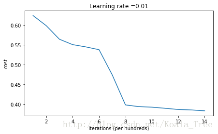

仔细观察会发现在第0代的损失是inf(无穷),这是由于数字舍入(numerical roundoff),使用更复杂的实现方法可以解决这个问题但是这不是我们关注的终点,现在忽略他就好。
总之,你看上去已经打破了对称,获得了更好的结果,模型不再对所有样本都预测为0:
print (predictions_train)
print (predictions_test)
plt.title("Model with large random initialization")
axes = plt.gca()
axes.set_xlim([-1.5,1.5])
axes.set_ylim([-1.5,1.5])
plot_decision_boundary(lambda x: predict_dec(parameters, x.T), train_X, train_Y)
经过观察可发现:
- 最开始的损失值很大,这是因为权重的初始化值很大,输出层的激活函数(sigmoid)输出的结果就很接近0或1,如果预测错了就会带来很大的loss(比如本来是0的预测值很接近1,损失就接近1),事实上,当
,损失接近无穷。
- 不好的初始化方式会导致梯度消失or梯度爆炸,更会拖累优化算法
- 如果你用更长的时间(提高迭代的轮数)训练这个网络你能看到更好地结果,但是用随机大值来初始化会让优化过程变慢
总结:
- 用随机大值初始化并不能work well
- 似乎用随机小值来初始化能得到更好地结果,但是有一个很重要的问题:多小才合适?(下一节介绍)
4 - He initialization
He的方法在上使用了一个(scaling factor)比例因子 sqrt(2./layers_dims[l-1]) 这是ReLu激活函数所需要的。
(He和“Xavier initialization”相似,不过后者用的是sqrt(1./layers_dims[l-1]))
练习:实现He初始化
# GRADED FUNCTION: initialize_parameters_he

def initialize_parameters_he(layers_dims):
    """
    Arguments:
    layer_dims -- python array (list) containing the size of each layer.

    Returns:
    parameters -- python dictionary containing your parameters "W1", "b1", ..., "WL", "bL":
                    W1 -- weight matrix of shape (layers_dims[1], layers_dims[0])
                    b1 -- bias vector of shape (layers_dims[1], 1)
                    ...
                    WL -- weight matrix of shape (layers_dims[L], layers_dims[L-1])
                    bL -- bias vector of shape (layers_dims[L], 1)
    """

    np.random.seed(3)
    parameters = {}
    L = len(layers_dims) - 1 # integer representing the number of layers

    for l in range(1, L + 1):
        ### START CODE HERE ### (≈ 2 lines of code)
        parameters['W' + str(l)] = np.random.randn(layers_dims[l],layers_dims[l-1])*np.sqrt(2./layers_dims[l-1])
        parameters['b' + str(l)] = np.zeros((layers_dims[l],1))
        ### END CODE HERE ###

    return parameters
parameters = initialize_parameters_he([2, 4, 1])
print("W1 = " + str(parameters["W1"]))
print("b1 = " + str(parameters["b1"]))
print("W2 = " + str(parameters["W2"]))
print("b2 = " + str(parameters["b2"]))W1 = [[ 1.78862847 0.43650985]
[ 0.09649747 -1.8634927 ]
[-0.2773882 -0.35475898]
[-0.08274148 -0.62700068]]
b1 = [[ 0.]
[ 0.]
[ 0.]
[ 0.]]
W2 = [[-0.03098412 -0.33744411 -0.92904268 0.62552248]]
b2 = [[ 0.]]运行下面代码得到结果
parameters = model(train_X, train_Y, initialization = "he")
print ("On the train set:")
predictions_train = predict(train_X, train_Y, parameters)
print ("On the test set:")
predictions_test = predict(test_X, test_Y, parameters)
Cost after iteration 0: 0.8830537463419761
Cost after iteration 1000: 0.6879825919728063
Cost after iteration 2000: 0.6751286264523371
Cost after iteration 3000: 0.6526117768893807
Cost after iteration 4000: 0.6082958970572938
Cost after iteration 5000: 0.5304944491717495
Cost after iteration 6000: 0.4138645817071794
Cost after iteration 7000: 0.3117803464844441
Cost after iteration 8000: 0.23696215330322562
Cost after iteration 9000: 0.18597287209206836
Cost after iteration 10000: 0.1501555628037182
Cost after iteration 11000: 0.12325079292273548
Cost after iteration 12000: 0.09917746546525937
Cost after iteration 13000: 0.0845705595402428
Cost after iteration 14000: 0.07357895962677366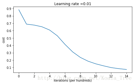
On the train set:
Accuracy: 0.993333333333
On the test set:
Accuracy: 0.96
plt.title("Model with He initialization")
axes = plt.gca()
axes.set_xlim([-1.5,1.5])
axes.set_ylim([-1.5,1.5])
plot_decision_boundary(lambda x: predict_dec(parameters, x.T), train_X, train_Y)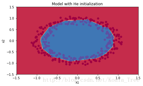
观察:
- He 初始化效果很好,只经过很少的迭代次数就能分开蓝色和红色点
5 - 总结
三种不同初始化的比较(迭代轮数和超参都相同):
| model | train accuracy | problem/comment |
| 3-layer NN with zeros initialization | 50% | fails to break symmetry |
| 3-layer NN with large random initialization | 83% | too large weights |
| 3-layer NN with He initialization | 99% | recommended method |
从上述实验中学到的知识:
- 不同的初始化会导致不同的结果
- 随机初始化被用来打破对称,确保不同的隐层神经元会学到不同的事
- 不要用太大的值来初始化W
- He 初始化是针对用ReLu做激活函数的神经网络
第二部分:正则化
首先导入你需要使用的库包
# import packages
import numpy as np
import matplotlib.pyplot as plt
from reg_utils import sigmoid, relu, plot_decision_boundary, initialize_parameters, load_2D_dataset, predict_dec
from reg_utils import compute_cost, predict, forward_propagation, backward_propagation, update_parameters
import sklearn
import sklearn.datasets
import scipy.io
from testCases import *

%matplotlib inline
plt.rcParams['figure.figsize'] = (7.0, 4.0) # set default size of plots
plt.rcParams['image.interpolation'] = 'nearest'
plt.rcParams['image.cmap'] = 'gray'
reg_utils.py中有一些重要的函数;
def initialize_parameters(layer_dims):
    """
    Arguments:
    layer_dims -- python array (list) containing the dimensions of each layer in our network

    Returns:
    parameters -- python dictionary containing your parameters "W1", "b1", ..., "WL", "bL":
                    W1 -- weight matrix of shape (layer_dims[l], layer_dims[l-1])
                    b1 -- bias vector of shape (layer_dims[l], 1)
                    Wl -- weight matrix of shape (layer_dims[l-1], layer_dims[l])
                    bl -- bias vector of shape (1, layer_dims[l])

    Tips:
    - For example: the layer_dims for the "Planar Data classification model" would have been [2,2,1].
    This means W1's shape was (2,2), b1 was (1,2), W2 was (2,1) and b2 was (1,1). Now you have to generalize it!
    - In the for loop, use parameters['W' + str(l)] to access Wl, where l is the iterative integer.
    """

    np.random.seed(3)
    parameters = {}
    L = len(layer_dims) # number of layers in the network

    for l in range(1, L):
        parameters['W' + str(l)] = np.random.randn(layer_dims[l], layer_dims[l-1]) / np.sqrt(layer_dims[l-1])
        parameters['b' + str(l)] = np.zeros((layer_dims[l], 1))

        assert(parameters['W' + str(l)].shape == layer_dims[l], layer_dims[l-1])
        assert(parameters['W' + str(l)].shape == layer_dims[l], 1)


    return parameters


def compute_cost(a3, Y):
    """
    Implement the cost function

    Arguments:
    a3 -- post-activation, output of forward propagation
    Y -- "true" labels vector, same shape as a3

    Returns:
    cost - value of the cost function
    """
    m = Y.shape[1]

    logprobs = np.multiply(-np.log(a3),Y) + np.multiply(-np.log(1 - a3), 1 - Y)
    cost = 1./m * np.nansum(logprobs)

    return cost


def load_2D_dataset():
    data = scipy.io.loadmat('datasets/data.mat')
    train_X = data['X'].T
    train_Y = data['y'].T
    test_X = data['Xval'].T
    test_Y = data['yval'].T

    plt.scatter(train_X[0, :], train_X[1, :], c=train_Y, s=40, cmap=plt.cm.Spectral);

    return train_X, train_Y, test_X, test_Y
最后一个函数中的数据集可以从这里下载:链接: https://pan.baidu.com/s/1epV9vHmp-u-tJNW_eMed2Q 提取码: ze7j
问题描述:你刚被法国队聘为AI专家,他们希望你推荐法国的守门员应该踢出球的位置这样法国球队的球员就可以用他们的头来击球了
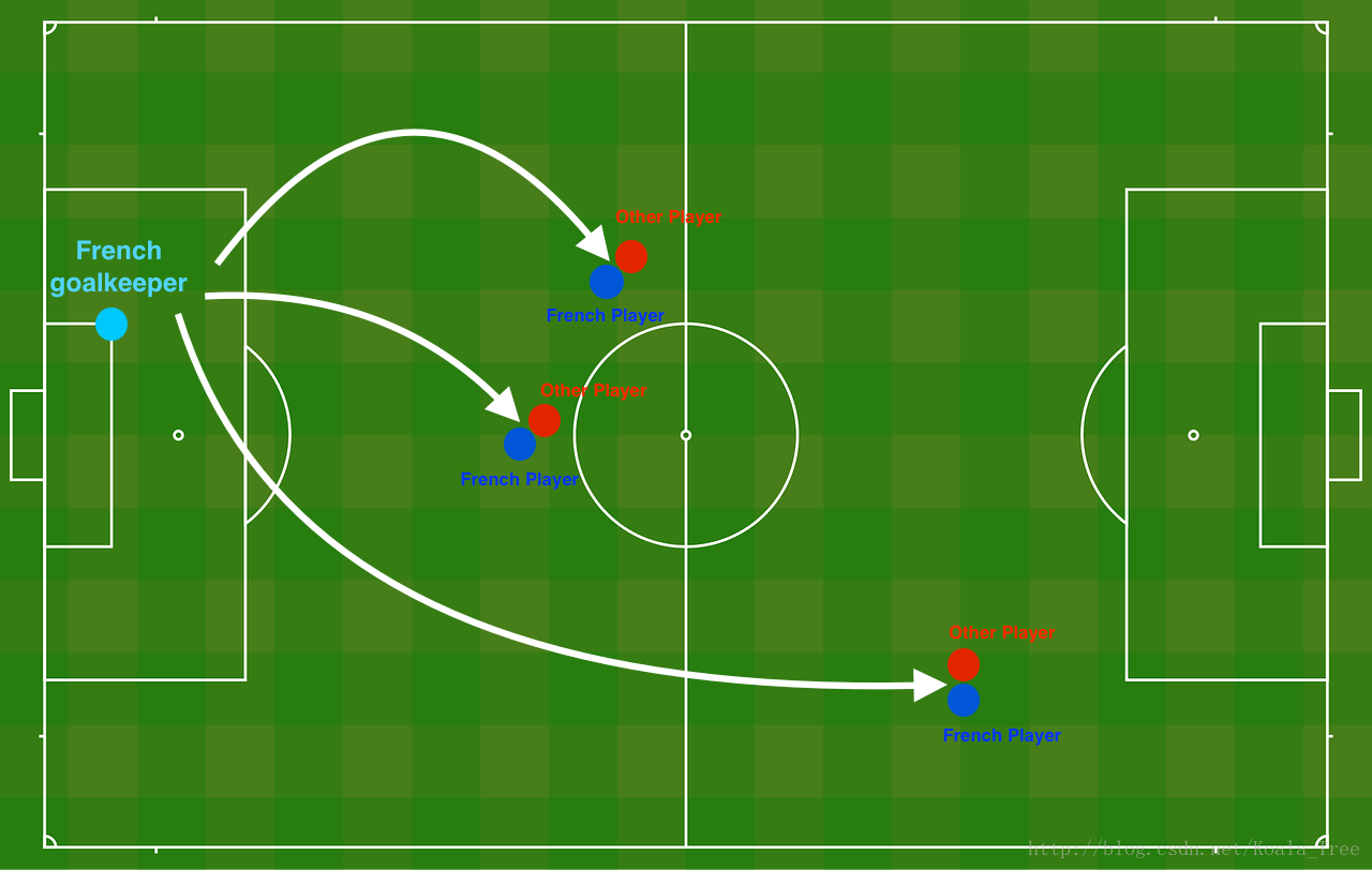
Figure 1 : Football field
守门员把球踢到空中,每个队的队员都在用他们的头顶球。
他们给你的是法国过去10场比赛的2D数据集:
train_X, train_Y, test_X, test_Y = load_2D_dataset()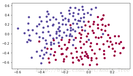
每个点都对应着足球场上的一个位置,法国守门员从足球场地的左边射出了球,而足球运动员在对应的位置用他/她的头击球。
- 蓝色点表示法国球员争顶成功
- 红点表示其他队的球员争顶成功
你的目标:使用一个深度学习模型来找到球场上的位置,守门员应该踢出球。
数据集分析:这个数据集有点噪声(noise),但它看起来像一条对角线,将左上角(蓝色)与右下半部分(红色)分隔开。
我们将首先尝试一个非正则化的模型。然后你将学习如何规范它并决定你将选择哪一种模式来解决法国足球公司的问题。
1 - Non-regularized model
你将会使用下面的神经网络模型(已经为你实现好了),他可以用在两种正则化模式中:
- in regularization mode 通过将lambd设置为一个非零值来使用。我们用“lambd”替代“lambda”是因为后者在py中是保留字
- in dropout mode 通过将keep_prob设置为一个小于1的值来使用。
你将会首先尝试没有正则化的模型,然后你需要依次实现:
- L2 regularization – functions: “
compute_cost_with_regularization()” and “backward_propagation_with_regularization()” - Dropout – functions: “
forward_propagation_with_dropout()” and “backward_propagation_with_dropout()”
仔细阅读下面代码,你需要理解他才能保证正确地调用你实现的函数
def model(X, Y, learning_rate = 0.3, num_iterations = 30000, print_cost = True, lambd = 0, keep_prob = 1):
    """
    Implements a three-layer neural network: LINEAR->RELU->LINEAR->RELU->LINEAR->SIGMOID.

    Arguments:
    X -- input data, of shape (input size, number of examples)
    Y -- true "label" vector (1 for blue dot / 0 for red dot), of shape (output size, number of examples)
    learning_rate -- learning rate of the optimization
    num_iterations -- number of iterations of the optimization loop
    print_cost -- If True, print the cost every 10000 iterations
    lambd -- regularization hyperparameter, scalar
    keep_prob - probability of keeping a neuron active during drop-out, scalar.

    Returns:
    parameters -- parameters learned by the model. They can then be used to predict.
    """

    grads = {}
    costs = []                            # to keep track of the cost
    m = X.shape[1]                        # number of examples
    layers_dims = [X.shape[0], 20, 3, 1]

    # Initialize parameters dictionary.
    parameters = initialize_parameters(layers_dims)

    # Loop (gradient descent)

    for i in range(0, num_iterations):

        # Forward propagation: LINEAR -> RELU -> LINEAR -> RELU -> LINEAR -> SIGMOID.
        if keep_prob == 1:
            a3, cache = forward_propagation(X, parameters)
        elif keep_prob < 1:
            a3, cache = forward_propagation_with_dropout(X, parameters, keep_prob)

        # Cost function
        if lambd == 0:
            cost = compute_cost(a3, Y)
        else:
            cost = compute_cost_with_regularization(a3, Y, parameters, lambd)

        # Backward propagation.
        assert(lambd==0 or keep_prob==1)    # it is possible to use both L2 regularization and dropout,
                                            # but this assignment will only explore one at a time
        if lambd == 0 and keep_prob == 1:
            grads = backward_propagation(X, Y, cache)
        elif lambd != 0:
            grads = backward_propagation_with_regularization(X, Y, cache, lambd)
        elif keep_prob < 1:
            grads = backward_propagation_with_dropout(X, Y, cache, keep_prob)

        # Update parameters.
        parameters = update_parameters(parameters, grads, learning_rate)

        # Print the loss every 10000 iterations
        if print_cost and i % 10000 == 0:
            print("Cost after iteration {}: {}".format(i, cost))
        if print_cost and i % 1000 == 0:
            costs.append(cost)

    # plot the cost
    plt.plot(costs)
    plt.ylabel('cost')
    plt.xlabel('iterations (x1,000)')
    plt.title("Learning rate =" + str(learning_rate))
    plt.show()

    return parameters
让我们开始在没有正则化的情况下训练模型并观察训练集和测试集上的acc
parameters = model(train_X, train_Y)
print ("On the training set:")
predictions_train = predict(train_X, train_Y, parameters)
print ("On the test set:")
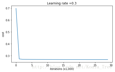
predictions_test = predict(test_X, test_Y, parameters)Cost after iteration 0: 0.6557412523481002
Cost after iteration 10000: 0.16329987525724216
Cost after iteration 20000: 0.13851642423255986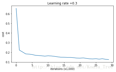
On the training set:
Accuracy: 0.947867298578
On the test set:
Accuracy: 0.915训练集的正确率为94.7%测试集是91.5%,这是baseline model (通过和baseline比较你将会观察到正则化对这个模型的影响),运行下面的代码绘制模型的决策边界。
plt.title("Model without regularization")
axes = plt.gca()
axes.set_xlim([-0.75,0.40])
axes.set_ylim([-0.75,0.65])
plot_decision_boundary(lambda x: predict_dec(parameters, x.T), train_X, train_Y)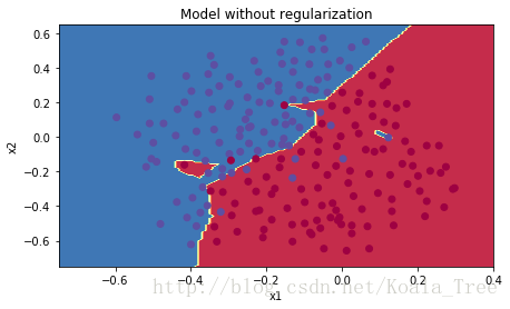
非正则化的模型很明显在训练集上出现了过拟合,他与噪声点也能匹配上(蓝色区域的红点),现在让我们用两种方法看看能不能减少这种过拟合。
2 - L2 Regularization
减少过拟合的标准方法是 L2正则化,它包括适当地修改你的成本函数:
从

到

让我们调整你的成本并观察其后果。
练习:实现函数 compute_cost_with_regularization() ,他可以计算第二个式子的cost,其中为了计算请使用
np.sum(np.square(Wl))注意这个操作你还需要对做,然后将三个部分加在一起并乘以
。
# GRADED FUNCTION: compute_cost_with_regularization

def compute_cost_with_regularization(A3, Y, parameters, lambd):
    """
    Implement the cost function with L2 regularization. See formula (2) above.

    Arguments:
    A3 -- post-activation, output of forward propagation, of shape (output size, number of examples)
    Y -- "true" labels vector, of shape (output size, number of examples)
    parameters -- python dictionary containing parameters of the model

    Returns:
    cost - value of the regularized loss function (formula (2))
    """
    m = Y.shape[1]
    W1 = parameters["W1"]
    W2 = parameters["W2"]
    W3 = parameters["W3"]

    cross_entropy_cost = compute_cost(A3, Y) # This gives you the cross-entropy part of the cost

    ### START CODE HERE ### (approx. 1 line)
    L2_regularization_cost = (1./m*lambd/2)*(np.sum(np.square(W1)) + np.sum(np.square(W2)) + np.sum(np.square(W3)))
    ### END CODER HERE ###

    cost = cross_entropy_cost + L2_regularization_cost

    return cost
先来用小的测试样例看看新的cost
A3, Y_assess, parameters = compute_cost_with_regularization_test_case()
print("cost = " + str(compute_cost_with_regularization(A3, Y_assess, parameters, lambd = 0.1)))
其中compute_cost_with_regularization_test_case()来自testcase.py具体如下,是预定义的值:
def compute_cost_with_regularization_test_case():
    np.random.seed(1)
    Y_assess = np.array([[1, 1, 0, 1, 0]])
    W1 = np.random.randn(2, 3)
    b1 = np.random.randn(2, 1)
    W2 = np.random.randn(3, 2)
    b2 = np.random.randn(3, 1)
    W3 = np.random.randn(1, 3)
    b3 = np.random.randn(1, 1)
    parameters = {"W1": W1, "b1": b1, "W2": W2, "b2": b2, "W3": W3, "b3": b3}
    a3 = np.array([[ 0.40682402,  0.01629284,  0.16722898,  0.10118111,  0.40682402]])
    return a3, Y_assess, parameters
结果:
cost = 1.78648594516当然,因为你改变了cost,因此对于反向传播过程同样需要改变,梯度的计算需要考虑到这些新的cost。
练习:实现反向传播中的带有正则化的梯度计算(仅仅有dW1, dW2 and dW3会发生变化),对于其中每一个权重矩阵,你需要加上正则化项的梯度
# GRADED FUNCTION: backward_propagation_with_regularization

def backward_propagation_with_regularization(X, Y, cache, lambd):
    """
    Implements the backward propagation of our baseline model to which we added an L2 regularization.

    Arguments:
    X -- input dataset, of shape (input size, number of examples)
    Y -- "true" labels vector, of shape (output size, number of examples)
    cache -- cache output from forward_propagation()
    lambd -- regularization hyperparameter, scalar

    Returns:
    gradients -- A dictionary with the gradients with respect to each parameter, activation and pre-activation variables
    """

    m = X.shape[1]
    (Z1, A1, W1, b1, Z2, A2, W2, b2, Z3, A3, W3, b3) = cache

    dZ3 = A3 - Y

    ### START CODE HERE ### (approx. 1 line)
    dW3 = 1./m * np.dot(dZ3, A2.T) + lambd/m * W3
    ### END CODE HERE ###
    db3 = 1./m * np.sum(dZ3, axis=1, keepdims = True)

    dA2 = np.dot(W3.T, dZ3)
    dZ2 = np.multiply(dA2, np.int64(A2 > 0))
    ### START CODE HERE ### (approx. 1 line)
    dW2 = 1./m * np.dot(dZ2, A1.T) + lambd/m * W2
    ### END CODE HERE ###
    db2 = 1./m * np.sum(dZ2, axis=1, keepdims = True)

    dA1 = np.dot(W2.T, dZ2)
    dZ1 = np.multiply(dA1, np.int64(A1 > 0))
    ### START CODE HERE ### (approx. 1 line)
    dW1 = 1./m * np.dot(dZ1, X.T) + lambd/m * W1
    ### END CODE HERE ###
    db1 = 1./m * np.sum(dZ1, axis=1, keepdims = True)

    gradients = {"dZ3": dZ3, "dW3": dW3, "db3": db3,"dA2": dA2,
                 "dZ2": dZ2, "dW2": dW2, "db2": db2, "dA1": dA1,
                 "dZ1": dZ1, "dW1": dW1, "db1": db1}

    return gradients
先通过一个小例子看看初始化的权重在什么数量级:
X_assess, Y_assess, cache = backward_propagation_with_regularization_test_case()

grads = backward_propagation_with_regularization(X_assess, Y_assess, cache, lambd = 0.7)
print ("dW1 = "+ str(grads["dW1"]))
print ("dW2 = "+ str(grads["dW2"]))
print ("dW3 = "+ str(grads["dW3"]))
dW1 = [[-0.25604646 0.12298827 -0.28297129]
[-0.17706303 0.34536094 -0.4410571 ]]
dW2 = [[ 0.79276486 0.85133918]
[-0.0957219 -0.01720463]
[-0.13100772 -0.03750433]]
dW3 = [[-1.77691347 -0.11832879 -0.09397446]]接下来让我们用的L2正则化来跑模型,函数 model()会调用
- compute_cost_with_regularization 而不是
compute_cost - backward_propagation_with_regularization 而不是 backward_propagation
执行:
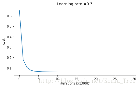
parameters = model(train_X, train_Y, lambd = 0.7)
print ("On the train set:")
predictions_train = predict(train_X, train_Y, parameters)
print ("On the test set:")
predictions_test = predict(test_X, test_Y, parameters)
得到结果:

恭喜,你的测试集正确率上升到了93%,你拯救了法国队,你的模型不再对训练集过拟合。让我们绘制出边界图:
plt.title("Model with L2-regularization")
axes = plt.gca()
axes.set_xlim([-0.75,0.40])
axes.set_ylim([-0.75,0.65])
plot_decision_boundary(lambda x: predict_dec(parameters, x.T), train_X, train_Y)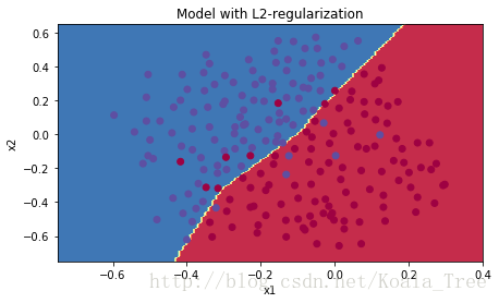
观察:
是一种超参,你可以根据验证集(dev set)的表现微调他(tuning)
- L2正则化使你的决策边界更平滑,如果lambda太大,可能会造成过平滑(oversmooth),这会导致模型有较高的偏差(high bias)
L2正则化到底做了什么?
l2-正则化依赖于这样的假设:一个小权重的模型比一个有大权重的模型更简单。因此,通过对成本函数中权重的平方值进行惩罚,你将所有的权重都推到更小的值上。由此获得较高的权重的成本太高了!这就导致了一个更平滑的模型:当输入发生变化时,输出的变化会更慢。
你应该记住的是 L2正则化的启示:
损失计算函数:
- 一个正规化的项被添加到成本中
反向传播函数:
- 关于权重矩阵在梯度方面有额外的项
权重衰减(weights decay):
- 权重被推到更小的值
3 - Dropout
最后,dropout是一种被广泛使用的正则化技术,专门用于深度学习。
它在每次迭代中随机关闭一些神经元。
当你关闭一些神经元时,你实际上就是在修改你的模型。dropout的出发点是,在每次迭代中,你训练一个不同的模型,它只使用你的神经元的一个子集。随着dropout,你的神经元对另一个特定神经元的激活变得不那么敏感,因为其他神经元可能在任何时候关闭。
3.1 - Forward propagation with dropout
练习:以dropout的方式实现向前传播。你使用的是一个3层的神经网络,将dropout添加到第一个和第二个隐藏图层中。我们不会将dropout应用到输入层或输出层。
说明:
你想要关闭第一层和第二层的一些神经元。要做到这一点,你将执行4个步骤:
- 在课堂上,我们讨论了如何创建一个变量
,它的维数与
相同,通过使用np.random.rand()随机地得到在0和1之间数字来初始化d。在这里,您将使用一个矢量化的实现,因此创建一个随机矩阵
,他和
有相同的维度
- 将上述随机初始化的值修改为true(1)和false(0),假设keep_prob=0.5,那么所有小于0.5的值都置1,大于0.5的值都置0。为了实现这个功能,你需要用到: X = (X < 0.5)
- 开始关键的shut down操作: 将
视为一个mask,让他和其他矩阵进行元素乘法就可以看做是关闭某些神经元,为此你需要将
- 输出恢复(或者 inverted dropout):让
# GRADED FUNCTION: forward_propagation_with_dropout

def forward_propagation_with_dropout(X, parameters, keep_prob = 0.5):
    """
    Implements the forward propagation: LINEAR -> RELU + DROPOUT -> LINEAR -> RELU + DROPOUT -> LINEAR -> SIGMOID.

    Arguments:
    X -- input dataset, of shape (2, number of examples)
    parameters -- python dictionary containing your parameters "W1", "b1", "W2", "b2", "W3", "b3":
                    W1 -- weight matrix of shape (20, 2)
                    b1 -- bias vector of shape (20, 1)
                    W2 -- weight matrix of shape (3, 20)
                    b2 -- bias vector of shape (3, 1)
                    W3 -- weight matrix of shape (1, 3)
                    b3 -- bias vector of shape (1, 1)
    keep_prob - probability of keeping a neuron active during drop-out, scalar

    Returns:
    A3 -- last activation value, output of the forward propagation, of shape (1,1)
    cache -- tuple, information stored for computing the backward propagation
    """

    np.random.seed(1)

    # retrieve parameters
    W1 = parameters["W1"]
    b1 = parameters["b1"]
    W2 = parameters["W2"]
    b2 = parameters["b2"]
    W3 = parameters["W3"]
    b3 = parameters["b3"]

    # LINEAR -> RELU -> LINEAR -> RELU -> LINEAR -> SIGMOID
    Z1 = np.dot(W1, X) + b1
    A1 = relu(Z1)
    ### START CODE HERE ### (approx. 4 lines)         # Steps 1-4 below correspond to the Steps 1-4 described above.
    D1 = np.random.rand(A1.shape[0],A1.shape[1])                                         # Step 1: initialize matrix D1 = np.random.rand(..., ...)
    D1 = D1 < keep_prob                                      # Step 2: convert entries of D1 to 0 or 1 (using keep_prob as the threshold)
    A1 = A1 * D1                                         # Step 3: shut down some neurons of A1
    A1 = A1 / keep_prob                                        # Step 4: scale the value of neurons that haven't been shut down
    ### END CODE HERE ###
    Z2 = np.dot(W2, A1) + b2
    A2 = relu(Z2)
    ### START CODE HERE ### (approx. 4 lines)
    D2 = np.random.rand(A2.shape[0],A2.shape[1])                                         # Step 1: initialize matrix D2 = np.random.rand(..., ...)
    D2 = D2 < keep_prob                                         # Step 2: convert entries of D2 to 0 or 1 (using keep_prob as the threshold)
    A2 = A2 * D2                                         # Step 3: shut down some neurons of A2
    A2 = A2 / keep_prob                                      # Step 4: scale the value of neurons that haven't been shut down
    ### END CODE HERE ###
    Z3 = np.dot(W3, A2) + b3
    A3 = sigmoid(Z3)

    cache = (Z1, D1, A1, W1, b1, Z2, D2, A2, W2, b2, Z3, A3, W3, b3)

    return A3, cache
用一个小例子看看A会变得怎么样:
X_assess, parameters = forward_propagation_with_dropout_test_case()
A3, cache = forward_propagation_with_dropout(X_assess, parameters, keep_prob = 0.7)
print ("A3 = " + str(A3))
A3 = [[ 0.36974721 0.00305176 0.04565099 0.49683389 0.36974721]]3.2 - Backward propagation with dropout
练习:实现有dropout的逆向传播。和以前一样,你正在训练一个3层的网络。在第一个和第二个隐藏层中添加dropout,使用存储在缓存中的D[1]和D[2]
说明:
实现有dropout的逆向传播很简单,只需要两步:
- 你在正向传播中随机关闭了一些神经元(通过
),在反向传播过程中,你同样需要关闭相同的神经元,此时
的mask
- 在向前传播过程中,你把A1除以keep_prob,在反向传播中,你必须再次用keep_prob来除dA1 (微积分的解释是,如果A1被keep_prob缩放,那么它的导数dA1也会被相同的keep_prob缩放)
# GRADED FUNCTION: backward_propagation_with_dropout

def backward_propagation_with_dropout(X, Y, cache, keep_prob):
    """
    Implements the backward propagation of our baseline model to which we added dropout.

    Arguments:
    X -- input dataset, of shape (2, number of examples)
    Y -- "true" labels vector, of shape (output size, number of examples)
    cache -- cache output from forward_propagation_with_dropout()
    keep_prob - probability of keeping a neuron active during drop-out, scalar

    Returns:
    gradients -- A dictionary with the gradients with respect to each parameter, activation and pre-activation variables
    """

    m = X.shape[1]
    (Z1, D1, A1, W1, b1, Z2, D2, A2, W2, b2, Z3, A3, W3, b3) = cache

    dZ3 = A3 - Y
    dW3 = 1./m * np.dot(dZ3, A2.T)
    db3 = 1./m * np.sum(dZ3, axis=1, keepdims = True)
    dA2 = np.dot(W3.T, dZ3)
    ### START CODE HERE ### (≈ 2 lines of code)
    dA2 = dA2 * D2              # Step 1: Apply mask D2 to shut down the same neurons as during the forward propagation
    dA2 = dA2 / keep_prob           # Step 2: Scale the value of neurons that haven't been shut down
    ### END CODE HERE ###
    dZ2 = np.multiply(dA2, np.int64(A2 > 0))
    dW2 = 1./m * np.dot(dZ2, A1.T)
    db2 = 1./m * np.sum(dZ2, axis=1, keepdims = True)

    dA1 = np.dot(W2.T, dZ2)
    ### START CODE HERE ### (≈ 2 lines of code)
    dA1 = dA1 * D1              # Step 1: Apply mask D1 to shut down the same neurons as during the forward propagation
    dA1 = dA1 / keep_prob             # Step 2: Scale the value of neurons that haven't been shut down
    ### END CODE HERE ###
    dZ1 = np.multiply(dA1, np.int64(A1 > 0))
    dW1 = 1./m * np.dot(dZ1, X.T)
    db1 = 1./m * np.sum(dZ1, axis=1, keepdims = True)

    gradients = {"dZ3": dZ3, "dW3": dW3, "db3": db3,"dA2": dA2,
                 "dZ2": dZ2, "dW2": dW2, "db2": db2, "dA1": dA1,
                 "dZ1": dZ1, "dW1": dW1, "db1": db1}

    return gradients
用一个小例子看看dA1和dA2的值:
X_assess, Y_assess, cache = backward_propagation_with_dropout_test_case()

gradients = backward_propagation_with_dropout(X_assess, Y_assess, cache, keep_prob = 0.8)

print ("dA1 = " + str(gradients["dA1"]))
print ("dA2 = " + str(gradients["dA2"]))
dA1 = [[ 0.36544439 0. -0.00188233 0. -0.17408748]
[ 0.65515713 0. -0.00337459 0. -0. ]]
dA2 = [[ 0.58180856 0. -0.00299679 0. -0.27715731]
[ 0. 0.53159854 -0. 0.53159854 -0.34089673]
[ 0. 0. -0.00292733 0. -0. ]]现在让我们用keep_prob = 0.86的dropout来训练model,这意味着在每一次迭代中你关闭了第1层和第2层的每一个神经元的概率是24%。函数model()会调用:
-forward_propagation_with_dropout instead of forward_propagation.
- backward_propagation_with_dropout instead of backward_propagation.
parameters = model(train_X, train_Y, keep_prob = 0.86, learning_rate = 0.3)

print ("On the train set:")
predictions_train = predict(train_X, train_Y, parameters)
print ("On the test set:")
predictions_test = predict(test_X, test_Y, parameters)
结果如下:

dropout工作很有效!测试集的准确性又提高了(到95%)!你的模特不会对训练集过拟合,在测试集中也表现出色。法国足球队将永远感激你!
运行下面的代码来绘制决策边界。
plt.title("Model with dropout")
axes = plt.gca()
axes.set_xlim([-0.75,0.40])
axes.set_ylim([-0.75,0.65])
plot_decision_boundary(lambda x: predict_dec(parameters, x.T), train_X, train_Y)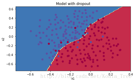
注意:
- 在使用dropout时,一个常见的错误是在训练模型和预测中使用它。只有在训练中,你应该使用dropout(随机删除节点),在predict时仍用原来的
forward_propagation。- 深度学习框架,如tensorflow、paddlepaddle、keras或caffe,都有一个dropout实现。不要紧张——你很快就会学到这些框架。
对于dropout你应该记住:
- 是一种正规化技术
- 你只能在训练中使用他。在测试(预测)期间不要使用dropout(随机删除节点)
- 在前向和反向传播中都要应用dropout
- 在训练期间,将每个使用了dropout的层都除以keep_prob,以保持激活的预期值不变。例如,如果keepprob是0.5,那么我们将平均关闭一半的节点,因此输出将被缩减到原来的0.5倍,因为只有剩下的一半对输出有贡献。除以0.5相当于乘以2。因此,现在的输出和原来的输出就具有了相同的期望值。
4 - Conclusions
结果比较:
| model | train acc | test acc |
| 3-layer NN without regularization | 95% | 91.5% |
| 3-layer NN with L2-regularization | 94% | 93% |
| 3-layer NN with dropout | 93% | 95% |
注意正则化会损害训练集的性能!这是因为它限制了网络在训练集中的能力,但是因为它最终提供了更好的测试精度,它正在帮助你的系统。
祝贺你完成这项任务!以及法国足球革命。:-)
我们想让你们记住的是:
- 正则化将帮助你减少过度拟合
- 正则化将使你的权重降低到更低的值
- L2的正则化和dropout是两种非常有效的正则化技术
第三部分 : 梯度检查
首先导入下面的包:
# Packages
import numpy as np
from testCases import *
from gc_utils import sigmoid, relu, dictionary_to_vector, vector_to_dictionary, gradients_to_vector
gc_utils.py的一些重要函数如下:
def dictionary_to_vector(parameters):
    """
    Roll all our parameters dictionary into a single vector satisfying our specific required shape.
    """
    keys = []
    count = 0
    for key in ["W1", "b1", "W2", "b2", "W3", "b3"]:

        # flatten parameter
        new_vector = np.reshape(parameters[key], (-1,1))
        keys = keys + [key]*new_vector.shape[0] #暂时用不到

        if count == 0:
            theta = new_vector
        else:
            theta = np.concatenate((theta, new_vector), axis=0)
        count = count + 1

    return theta, keys


def vector_to_dictionary(theta):
    """
    Unroll all our parameters dictionary from a single vector satisfying our specific required shape.
    """
    parameters = {}
    parameters["W1"] = theta[:20].reshape((5,4))
    parameters["b1"] = theta[20:25].reshape((5,1))
    parameters["W2"] = theta[25:40].reshape((3,5))
    parameters["b2"] = theta[40:43].reshape((3,1))
    parameters["W3"] = theta[43:46].reshape((1,3))
    parameters["b3"] = theta[46:47].reshape((1,1))

    return parameters


def gradients_to_vector(gradients):
    """
    Roll all our gradients dictionary into a single vector satisfying our specific required shape.
    """

    count = 0
    for key in ["dW1", "db1", "dW2", "db2", "dW3", "db3"]:
        # flatten parameter
        new_vector = np.reshape(gradients[key], (-1,1))

        if count == 0:
            theta = new_vector
        else:
            theta = np.concatenate((theta, new_vector), axis=0)
        count = count + 1

    return theta
1. How does gradient checking work?
后向传播计算梯度,其中theda表示模型的参数,J是用正向传播(得到A3)和损失函数(得到cost)计算的。
因为前向传播相对容易实现,你有信心你做对了,所以你几乎百分百确定你计算的成本J是正确的,因此,您可以使用您的代码来计算J,并用来验证计算的代码。
让我们回顾一下导数(或梯度)的数值逼近的定义:

我们知道下面的内容:
是你想要验证是否被正确计算的值
- 你可以计算
和
(在这个例子中theda是一个实数),因为你确信你对J的计算是正确的
让我们用上面的计算公式和一个小值来验证你对
的计算。
2. 1-dimensional gradient checking
考虑一维线性函数,该模型只包含一个实值参数theda,并将x作为输入。
您将实现代码来计算J(.)和它的导数的计算。然后你将使用梯度检查来确保你对J的微分计算是正确的。
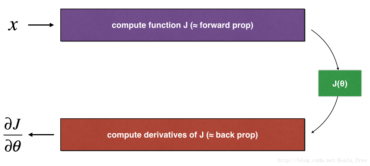
Figure 1 : 1D linear model
上面的图表显示了关键的计算步骤:首先从x开始,然后评估函数J(x)(“前向传播”)。然后计算导数(“反向传播”)。
练习:在两个单独的函数中为这个简单的过程实现“前向传播”和“反向传播”。即计算J(.)(“前向传播”)和它对theda的导数(“反向传播”)。
# GRADED FUNCTION: forward_propagation

def forward_propagation(x, theta):
    """
    Implement the linear forward propagation (compute J) presented in Figure 1 (J(theta) = theta * x)

    Arguments:
    x -- a real-valued input
    theta -- our parameter, a real number as well

    Returns:
    J -- the value of function J, computed using the formula J(theta) = theta * x
    """

    ### START CODE HERE ### (approx. 1 line)
    J = theta * x
    ### END CODE HERE ###

    return J
x, theta = 2, 4
J = forward_propagation(x, theta)
print ("J = " + str(J))J = 8练习: 现在,实现图1的向后传播步骤(导数计算)。也就是,计算对theda的导数。
# GRADED FUNCTION: backward_propagation

def backward_propagation(x, theta):
    """
    Computes the derivative of J with respect to theta (see Figure 1).

    Arguments:
    x -- a real-valued input
    theta -- our parameter, a real number as well

    Returns:
    dtheta -- the gradient of the cost with respect to theta
    """

    ### START CODE HERE ### (approx. 1 line)
    dtheta = x
    ### END CODE HERE ###

    return dtheta
x, theta = 2, 4
dtheta = backward_propagation(x, theta)
print ("dtheta = " + str(dtheta))dtheta = 2练习:为了证明backward_propagation()函数正确地计算了梯度我们来实现梯度检查。
说明:
- 首先计算gradapprox,步骤如下:

- 然后使用反向传播来计算gradients,并将结果存储在一个变量“grad”中
- 最后,使用以下公式计算“gradapprox”和“grad”之间的相对差异:

你需要三部来计算上面的式子:
- 用np.linalg.norm()来计算分子。
- 计算分母,您将需要调用np.linalg.norm()两次。
- 两者相除。
如果这个差异很小(比如小于1e-7),您就可以很有把握地认为您正确计算出了梯度。否则,在梯度计算中可能会出现错误。
# GRADED FUNCTION: gradient_check

def gradient_check(x, theta, epsilon = 1e-7):
    """
    Implement the backward propagation presented in Figure 1.

    Arguments:
    x -- a real-valued input
    theta -- our parameter, a real number as well
    epsilon -- tiny shift to the input to compute approximated gradient with formula(1)

    Returns:
    difference -- difference (2) between the approximated gradient and the backward propagation gradient
    """

    # Compute gradapprox using left side of formula (1). epsilon is small enough, you don't need to worry about the limit.
    ### START CODE HERE ### (approx. 5 lines)
    thetaplus = theta + epsilon                               # Step 1
    thetaminus = theta - epsilon                              # Step 2
    J_plus = forward_propagation(x, thetaplus)                                  # Step 3
    J_minus = forward_propagation(x, thetaminus)                                 # Step 4
    gradapprox = (J_plus - J_minus) / (2 * epsilon)                              # Step 5
    ### END CODE HERE ###

    # Check if gradapprox is close enough to the output of backward_propagation()
    ### START CODE HERE ### (approx. 1 line)
    grad = backward_propagation(x, theta)
    ### END CODE HERE ###

    ### START CODE HERE ### (approx. 1 line)
    numerator = np.linalg.norm(grad - gradapprox)                               # Step 1'
    denominator = np.linalg.norm(grad) + np.linalg.norm(gradapprox)                            # Step 2'
    difference = numerator / denominator                              # Step 3'
    ### END CODE HERE ###

    if difference < 1e-7:
        print ("The gradient is correct!")
    else:
        print ("The gradient is wrong!")

    return difference
x, theta = 2, 4
difference = gradient_check(x, theta)
print("difference = " + str(difference))The gradient is correct!
difference = 2.91933588329e-10恭喜,差值比阈值小。因此,您可以非常确信您已经正确地计算了backward_propagation()中的梯度。
现在,在更一般的情况下,你的成本函数J有不止一个一维的输入。当你在训练一个神经网络时,实际上是由多个矩阵组成的W[ l ]和偏差b[ l ]!重要的是要知道如何对高维输入进行梯度检查。让我们解决它!
3. N-dimensional gradient checking
下图描述了您的欺诈检测模型的向前和向后传播。

Figure 2 : deep neural network
LINEAR -> RELU -> LINEAR -> RELU -> LINEAR -> SIGMOID
让我们看一下向前传播和反向传播的实现。
def forward_propagation_n(X, Y, parameters):
    """
    Implements the forward propagation (and computes the cost) presented in Figure 3.

    Arguments:
    X -- training set for m examples
    Y -- labels for m examples
    parameters -- python dictionary containing your parameters "W1", "b1", "W2", "b2", "W3", "b3":
                    W1 -- weight matrix of shape (5, 4)
                    b1 -- bias vector of shape (5, 1)
                    W2 -- weight matrix of shape (3, 5)
                    b2 -- bias vector of shape (3, 1)
                    W3 -- weight matrix of shape (1, 3)
                    b3 -- bias vector of shape (1, 1)

    Returns:
    cost -- the cost function (logistic cost for one example)
    """

    # retrieve parameters
    m = X.shape[1]
    W1 = parameters["W1"]
    b1 = parameters["b1"]
    W2 = parameters["W2"]
    b2 = parameters["b2"]
    W3 = parameters["W3"]
    b3 = parameters["b3"]

    # LINEAR -> RELU -> LINEAR -> RELU -> LINEAR -> SIGMOID
    Z1 = np.dot(W1, X) + b1
    A1 = relu(Z1)
    Z2 = np.dot(W2, A1) + b2
    A2 = relu(Z2)
    Z3 = np.dot(W3, A2) + b3
    A3 = sigmoid(Z3)

    # Cost
    logprobs = np.multiply(-np.log(A3),Y) + np.multiply(-np.log(1 - A3), 1 - Y)
    cost = 1./m * np.sum(logprobs)

    cache = (Z1, A1, W1, b1, Z2, A2, W2, b2, Z3, A3, W3, b3)

    return cost, cache
backward propagation:
def backward_propagation_n(X, Y, cache):
    """
    Implement the backward propagation presented in figure 2.

    Arguments:
    X -- input datapoint, of shape (input size, 1)
    Y -- true "label"
    cache -- cache output from forward_propagation_n()

    Returns:
    gradients -- A dictionary with the gradients of the cost with respect to each parameter, activation and pre-activation variables.
    """

    m = X.shape[1]
    (Z1, A1, W1, b1, Z2, A2, W2, b2, Z3, A3, W3, b3) = cache

    dZ3 = A3 - Y
    dW3 = 1./m * np.dot(dZ3, A2.T)
    db3 = 1./m * np.sum(dZ3, axis=1, keepdims = True)

    dA2 = np.dot(W3.T, dZ3)
    dZ2 = np.multiply(dA2, np.int64(A2 > 0))
    dW2 = 1./m * np.dot(dZ2, A1.T) * 2
    db2 = 1./m * np.sum(dZ2, axis=1, keepdims = True)

    dA1 = np.dot(W2.T, dZ2)
    dZ1 = np.multiply(dA1, np.int64(A1 > 0))
    dW1 = 1./m * np.dot(dZ1, X.T)
    db1 = 4./m * np.sum(dZ1, axis=1, keepdims = True)

    gradients = {"dZ3": dZ3, "dW3": dW3, "db3": db3,
                 "dA2": dA2, "dZ2": dZ2, "dW2": dW2, "db2": db2,
                 "dA1": dA1, "dZ1": dZ1, "dW1": dW1, "db1": db1}

    return gradients
您在欺诈检测测试集上获得了一些结果,但是您不能完全确定您的模型。没有人是完美的!让我们实现梯度检查,以验证您的梯度是否正确。
How does gradient checking work?.
如1)和2),您需要将“gradapprox”与反向传播计算的梯度进行比较。这个公式仍然是:

然而,theta不再是一个标量。它是一个叫做“parameters”的字典。我们为您实现了一个名为dictionary_to_vector()的函数。它将“parameters”字典转换成一个称为“values”的向量.(通过将所有参数(W1、b1、W2、b2、W3、b3)转换成矢量并将它们连接起来)。
他的逆函数是“vector_to_dictionary()”,它会将新矢量重新转换回原来的状态然后输出“parameters”字典。
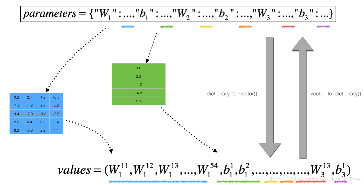
Figure 2 : dictionary_to_vector() and vector_to_dictionary()
You will need these functions in gradient_check_n()
我们还使用 gradients_to_vector() 将“gradients”字典转换成一个向量“grad”。你不需要担心这个。
练习:实现函数 gradient_check_n()
说明:
由于cost是一个标量,J()函数的结果可以认为是由cost组成的向量 [ cost,cost,...,cost ] ,有多少个参数就有多少个cost,每个cost的值都一样(可以理解为每个参数都是用相同的样本来训练的,因此每个参数的cost都相同,都等于整体的cost),这样我们就可以将一个多维问题转化为一个一维问题,利用上一节的方法,循环计算每一个参数的diff
下面是一些可以帮助您实现梯度检查的伪代码:
假设参数共有num_parameters个则

因此,你得到一个向量gradapprox,在这里,gradappro[i]是关于第i个参数的梯度 parameter_values[i] 的近似值。现在你可以将这个梯度向量与反向传播的梯度向量进行比较。就像一维的情况(步骤1',2',3'),计算:

# GRADED FUNCTION: gradient_check_n

def gradient_check_n(parameters, gradients, X, Y, epsilon = 1e-7):
    """
    Checks if backward_propagation_n computes correctly the gradient of the cost output by forward_propagation_n

    Arguments:
    parameters -- python dictionary containing your parameters "W1", "b1", "W2", "b2", "W3", "b3":
    grad -- output of backward_propagation_n, contains gradients of the cost with respect to the parameters.
    x -- input datapoint, of shape (input size, 1)
    y -- true "label"
    epsilon -- tiny shift to the input to compute approximated gradient with formula(1)

    Returns:
    difference -- difference (2) between the approximated gradient and the backward propagation gradient
    """

    # Set-up variables
    parameters_values, _ = dictionary_to_vector(parameters)
    grad = gradients_to_vector(gradients)
    num_parameters = parameters_values.shape[0]
    J_plus = np.zeros((num_parameters, 1))
    J_minus = np.zeros((num_parameters, 1))
    gradapprox = np.zeros((num_parameters, 1))

    # Compute gradapprox
    for i in range(num_parameters):

        # Compute J_plus[i]. Inputs: "parameters_values, epsilon". Output = "J_plus[i]".
        # "_" is used because the function you have to outputs two parameters but we only care about the first one
        ### START CODE HERE ### (approx. 3 lines)
        thetaplus = np.copy(parameters_values)                                      # Step 1
        thetaplus[i][0] = thetaplus[i][0] + epsilon                                # Step 2
        J_plus[i], _ = forward_propagation_n(X, Y, vector_to_dictionary(thetaplus))                                  # Step 3
        ### END CODE HERE ###

        # Compute J_minus[i]. Inputs: "parameters_values, epsilon". Output = "J_minus[i]".
        ### START CODE HERE ### (approx. 3 lines)
        thetaminus = np.copy(parameters_values)                                     # Step 1
        thetaminus[i][0] = thetaminus[i][0] - epsilon                            # Step 2
        J_minus[i], _ = forward_propagation_n(X, Y, vector_to_dictionary(thetaminus))                                  # Step 3
        ### END CODE HERE ###

        # Compute gradapprox[i]
        ### START CODE HERE ### (approx. 1 line)
        gradapprox[i] = (J_plus[i] - J_minus[i]) / (2.* epsilon)
        ### END CODE HERE ###

    # Compare gradapprox to backward propagation gradients by computing difference.
    ### START CODE HERE ### (approx. 1 line)
    numerator = np.linalg.norm(grad - gradapprox)                                           # Step 1'
    denominator = np.linalg.norm(grad) + np.linalg.norm(gradapprox)                                         # Step 2'
    difference = numerator / denominator                                          # Step 3'
    ### END CODE HERE ###

    if difference > 1e-7:
        print ("\033[93m" + "There is a mistake in the backward propagation! difference = " + str(difference) + "\033[0m")
    else:
        print ("\033[92m" + "Your backward propagation works perfectly fine! difference = " + str(difference) + "\033[0m")

    return difference
X, Y, parameters = gradient_check_n_test_case()#自定义的简易数据集
cost, cache = forward_propagation_n(X, Y, parameters)
gradients = backward_propagation_n(X, Y, cache)
difference = gradient_check_n(parameters, gradients, X, Y)得到结果:

似乎我们给你的 backward_propagation_n() 代码中有错误!很好,你已经实现了梯度检查。回到backward_propagation,并尝试查找/纠正错误(提示:检查dW2和db1)。当你认为你已经修复了它的时候,重新运行梯度检查。
正确的 backward_propagation_n():
def backward_propagation_n_right(X, Y, cache):
    """
    Implement the backward propagation presented in figure 2.

    Arguments:
    X -- input datapoint, of shape (input size, 1)
    Y -- true "label"
    cache -- cache output from forward_propagation_n()

    Returns:
    gradients -- A dictionary with the gradients of the cost with respect to each parameter, activation and pre-activation variables.
    """

    m = X.shape[1]
    (Z1, A1, W1, b1, Z2, A2, W2, b2, Z3, A3, W3, b3) = cache

    dZ3 = A3 - Y
    dW3 = 1./m * np.dot(dZ3, A2.T)
    db3 = 1./m * np.sum(dZ3, axis=1, keepdims = True)

    dA2 = np.dot(W3.T, dZ3)
    dZ2 = np.multiply(dA2, np.int64(A2 > 0))
    dW2 = 1./m * np.dot(dZ2, A1.T)
    db2 = 1./m * np.sum(dZ2, axis=1, keepdims = True)

    dA1 = np.dot(W2.T, dZ2)
    dZ1 = np.multiply(dA1, np.int64(A1 > 0))
    dW1 = 1./m * np.dot(dZ1, X.T)
    db1 = 1./m * np.sum(dZ1, axis=1, keepdims = True)

    gradients = {"dZ3": dZ3, "dW3": dW3, "db3": db3,
                 "dA2": dA2, "dZ2": dZ2, "dW2": dW2, "db2": db2,
                 "dA1": dA1, "dZ1": dZ1, "dW1": dW1, "db1": db1}

    return gradients
结果:

Note:
- 梯度检查很慢!近似的梯度
计算成本很高。由于这个原因,我们在训练期间不进行每次迭代的梯度检查。只需在几次迭代中检查这个梯度是否正确。
- 梯度检查,至少像我们展示的那样,并不适用于dropout。你通常会在没有dropout的情况下运行梯度检查算法,以确保你的后推是正确的,然后再加上dropout。
我们想让你明白:
- 梯度检查计算了从反向传播的梯度与梯度的数值近似的梯度(利用正向传播计算)之间的距离。
- 梯度检查是缓慢的,所以我们不会在每次训练的迭代中运行它。你通常只运行它来确保你的代码是正确的,然后关闭它并进行实际的学习过程