P0 前言

第一门课 : 神经网络与深度学习
第四周 : Deep Neural Networks（深层神经网络）
主要知识点 : 深度神经网络、DNN的前向和反向传播（Forward & Backward propagation）、参数和超参数等

视频地址：https://mooc.study.163.com/learn/2001281002?tid=2001392029#/learn/announce

笔记地址：

数据集+作业源码+本地版作业网页下载：链接：https://pan.baidu.com/s/1htHH4FSlryxirxW4gLS82w
提取码：r9ob

P1 作业

Part-1 ：逐步建立你的深层神经网络

1-Packages

让我们首先导入在这个作业中需要的所有包。

import numpy as np
import h5py
import matplotlib.pyplot as plt
from testCases_v3 import *
from dnn_utils_v2 import sigmoid, sigmoid_backward, relu, relu_backward

%matplotlib inline
plt.rcParams['figure.figsize'] = (5.0, 4.0) # set default size of plots
plt.rcParams['image.interpolation'] = 'nearest'
plt.rcParams['image.cmap'] = 'gray'

%load_ext autoreload
%autoreload 2

np.random.seed(1)

其中dnn_utils_v2.py中包含了一些重要函数如下所示：

sigmoid函数：

def sigmoid(Z):
    """
    Implements the sigmoid activation in numpy

    Arguments:
    Z -- numpy array of any shape

    Returns:
    A -- output of sigmoid(z), same shape as Z
    cache -- returns Z as well, useful during backpropagation
    """

    A = 1/(1+np.exp(-Z))
    cache = Z

    return A, cache

反向传播中sigmoid函数：

def sigmoid_backward(dA, cache):
    """
    Implement the backward propagation for a single SIGMOID unit.

    Arguments:
    dA -- post-activation gradient, of any shape
    cache -- 'Z' where we store for computing backward propagation efficiently

    Returns:
    dZ -- Gradient of the cost with respect to Z
    """

    Z = cache

    s = 1/(1+np.exp(-Z))
    dZ = dA * s * (1-s)

    assert (dZ.shape == Z.shape)

    return dZ

Relu函数：

def relu(Z):
    """
    Implement the RELU function.

    Arguments:
    Z -- Output of the linear layer, of any shape

    Returns:
    A -- Post-activation parameter, of the same shape as Z
    cache -- a python dictionary containing "A" ; stored for computing the backward pass efficiently
    """

    A = np.maximum(0,Z)

    assert(A.shape == Z.shape)

    cache = Z 
    return A, cache

反向传播中的ReLu函数：

def relu_backward(dA, cache):
    """
    Implement the backward propagation for a single RELU unit.

    Arguments:
    dA -- post-activation gradient, of any shape
    cache -- 'Z' where we store for computing backward propagation efficiently

    Returns:
    dZ -- Gradient of the cost with respect to Z
    """

    Z = cache
    dZ = np.array(dA, copy=True) # just converting dz to a correct object.

    # When z <= 0, you should set dz to 0 as well. 
    dZ[Z <= 0] = 0

    assert (dZ.shape == Z.shape)

    return dZ

2-作业大纲

要构建您的神经网络，您将实现几个“辅助函数”。这些辅助函数将在下次作业中用于构建一个双层神经网络和l层神经网络。您将实现的每个小助手函数都有详细的说明，这些说明将指导您完成必要的步骤。以下是这份作业的大纲，你可以:

初始化两层网络和l层神经网络的参数。initialization（）
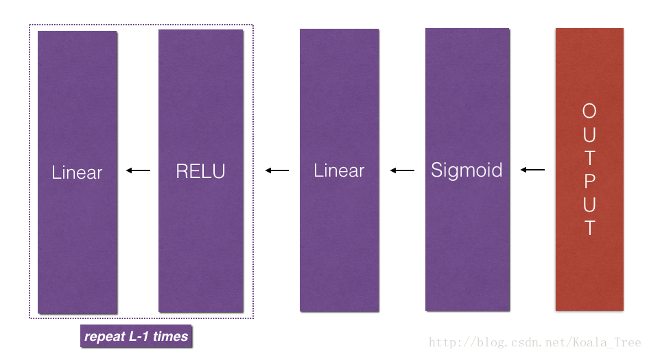
实现正向传播模块(如下图紫色所示)。

完成一个层的正向传播步骤的线性部分（产生 $Z^{[l]}$ ）linear_forward()

激活函数（sigmoid/Relu）我们已经帮你实现好了

将上面两步进行结合从而得到一个新的函数 linear_activation_forward()

重复 linear_activation_forward(Relu)函数 L-1次（针对第一层到第L-1层）然后再进行一次 linear_activation_forward(sigmoid)函数（针对最后一层），这样你会得到一个新的函数 L_model_forward（）

计算loss compute_cost()
实现反向传播模块（如下图红色所示）

完成向后传播步骤的线性部分。linear_backward()

我们已经实现了ACTIVATE函数的梯度(relu_reverse / sigmoid_reverse)

将上面两步进行结合从而得到一个新的函数 linear_activation_backward()

先进行一次linear_activation_backward(sigmoid)，然后重复L-1次linear_activation_backward(Relu)从而得到新函数L_model_backward（）

最终更新参数 update_parameters()

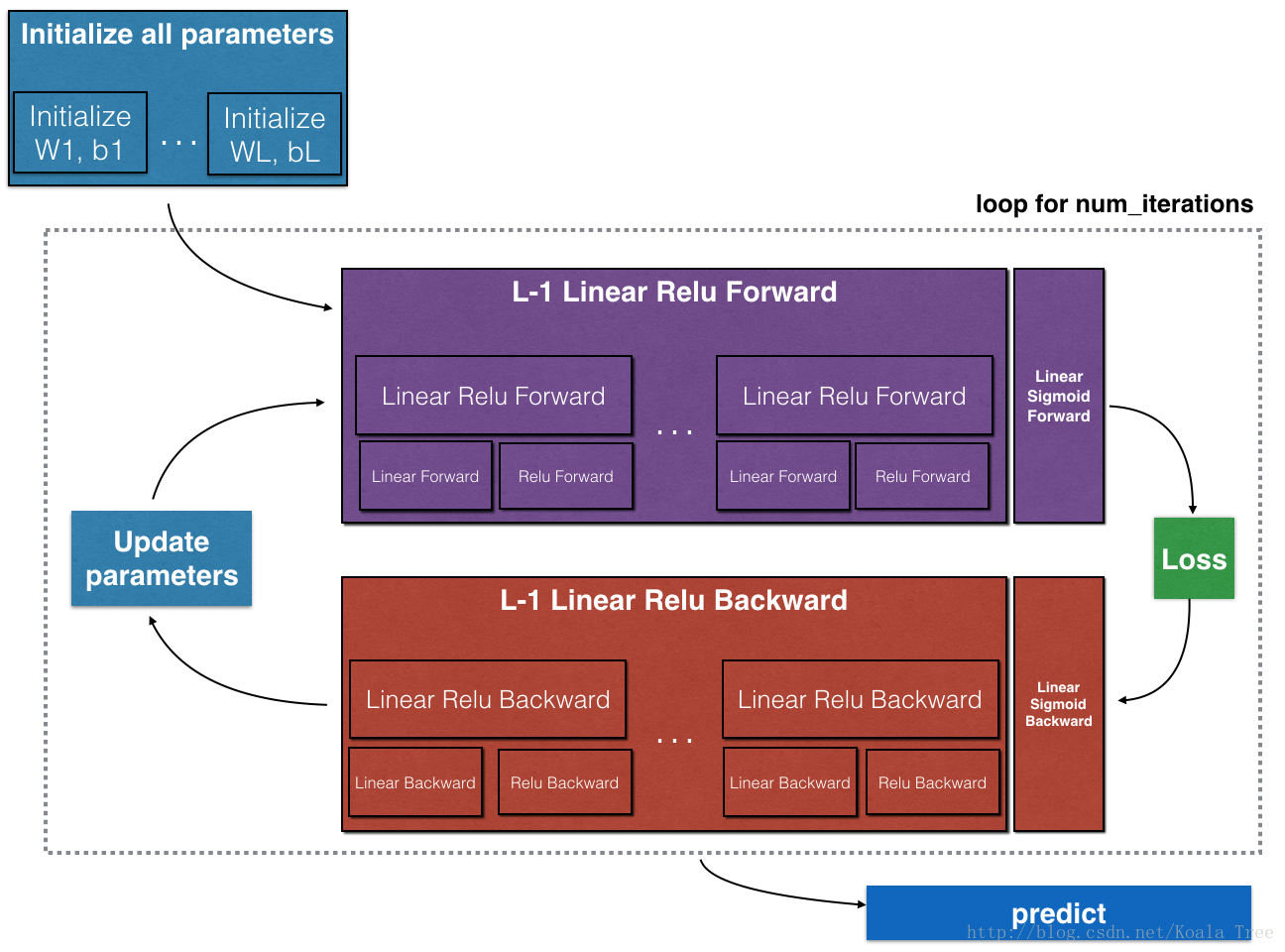
注意，对于每个正向函数，都有相应的反向函数。这就是为什么在forward模块的每个步骤中都要将一些值存储在缓存中。缓存的值对于计算梯度非常有用。在backpropagation模块中，您将使用缓存来计算梯度。这个作业将向你展示如何执行这些步骤。

3-初始化

您将编写两个助手函数，用于初始化模型的参数。第一个函数将用于初始化两个层模型的参数。第二个将把这个初始化过程推广到L层。

3.1 - 两层神经网络

练习: 创建并初始化2层神经网络的参数

说明：

两层神经网路的结构是：LINEAR -> RELU -> LINEAR -> SIGMOID
对权重矩阵使用随机初始化 np.random.randn(shape)*0.01
对偏差使用零初始化 np.zeros(shape)

# GRADED FUNCTION: initialize_parameters

def initialize_parameters(n_x, n_h, n_y):
    """
    Argument:
    n_x -- size of the input layer
    n_h -- size of the hidden layer
    n_y -- size of the output layer

    Returns:
    parameters -- python dictionary containing your parameters:
                    W1 -- weight matrix of shape (n_h, n_x)
                    b1 -- bias vector of shape (n_h, 1)
                    W2 -- weight matrix of shape (n_y, n_h)
                    b2 -- bias vector of shape (n_y, 1)
    """

    np.random.seed(1)

    ### START CODE HERE ### (≈ 4 lines of code)
    W1 = np.random.randn(n_h, n_x)*0.01
    b1 = np.zeros((n_h, 1))
    W2 = np.random.randn(n_y, n_h)*0.01
    b2 = np.zeros((n_y, 1))
    ### END CODE HERE ###

    assert(W1.shape == (n_h, n_x))
    assert(b1.shape == (n_h, 1))
    assert(W2.shape == (n_y, n_h))
    assert(b2.shape == (n_y, 1))

    parameters = {"W1": W1,
                  "b1": b1,
                  "W2": W2,
                  "b2": b2}

    return parameters

parameters = initialize_parameters(3,2,1)
print("W1 = " + str(parameters["W1"]))
print("b1 = " + str(parameters["b1"]))
print("W2 = " + str(parameters["W2"]))
print("b2 = " + str(parameters["b2"]))

W1 = [[ 0.01624345 -0.00611756 -0.00528172]
 [-0.01072969  0.00865408 -0.02301539]]
b1 = [[ 0.]
 [ 0.]]
W2 = [[ 0.01744812 -0.00761207]]
b2 = [[ 0.]]

3.2- L层神经网络

较深的l层神经网络的初始化更为复杂，因为有更多的权值矩阵和偏置向量。在完成initialize_parameters_deep时，应该确保每个层之间的维度匹配。

例如输入X是（12288,209）维的（也就是说有m=209个样本），那么：

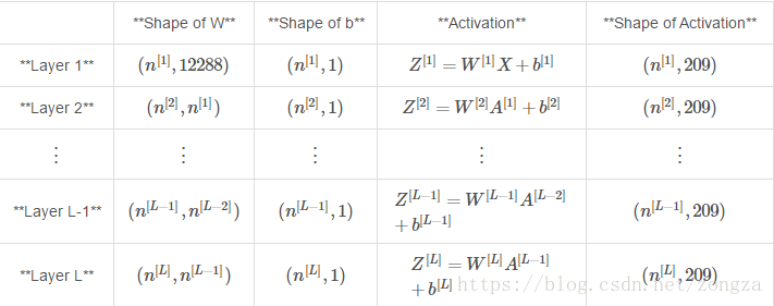
公式计算如下所示：

$W = \begin{bmatrix} j & k & l\\ m & n & o \\ p & q & r \end{bmatrix}\;\;\; X = \begin{bmatrix} a & b & c\\ d & e & f \\ g & h & i \end{bmatrix} \;\;\; b =\begin{bmatrix} s \\ t \\ u \end{bmatrix}\tag{2}$

$WX + b = \begin{bmatrix} (ja + kd + lg) + s & (jb + ke + lh) + s & (jc + kf + li)+ s\\ (ma + nd + og) + t & (mb + ne + oh) + t & (mc + nf + oi) + t\\ (pa + qd + rg) + u & (pb + qe + rh) + u & (pc + qf + ri)+ u \end{bmatrix}\tag{3}$

练习:实现l层神经网络的初始化。

说明：

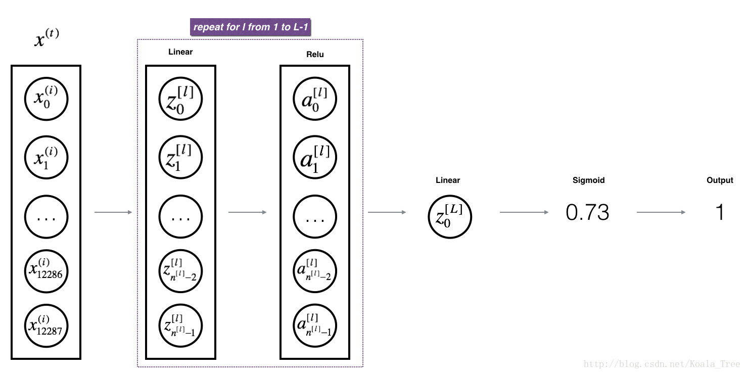
模型的结构是： [LINEAR -> RELU] × (L-1) -> LINEAR -> SIGMOID 它有L−1 层使用ReLU激活函数后面跟着一个输出层使用sigmoid激活函数。
对权重矩阵使用随机初始化 np.random.randn(shape)*0.01
对偏差使用零初始化 np.zeros(shape)
我们将在一个变量layer_dims中存储n[l]（即不同层中的单位数量）例如layer_dim=[n_x,n_h,n_y]

下面是L=1(一层神经网络)的实现。它应该会启发您实现通用的案例(l层神经网络)。

  if L == 1:
        parameters["W" + str(L)] = np.random.randn(layer_dims[1], layer_dims[0]) * 0.01
        parameters["b" + str(L)] = np.zeros((layer_dims[1], 1))

# GRADED FUNCTION: initialize_parameters_deep

def initialize_parameters_deep(layer_dims):
    """
    Arguments:
    layer_dims -- python array (list) containing the dimensions of each layer in our network

    Returns:
    parameters -- python dictionary containing your parameters "W1", "b1", ..., "WL", "bL":
                    Wl -- weight matrix of shape (layer_dims[l], layer_dims[l-1])
                    bl -- bias vector of shape (layer_dims[l], 1)
    """

    np.random.seed(3)
    parameters = {}
    L = len(layer_dims)            # number of layers in the network

    for l in range(1, L):
        ### START CODE HERE ### (≈ 2 lines of code)
        parameters['W' + str(l)] = np.random.randn(layer_dims[l], layer_dims[l-1])*0.01
        parameters['b' + str(l)] = np.zeros((layer_dims[l], 1))
        ### END CODE HERE ###

        assert(parameters['W' + str(l)].shape == (layer_dims[l], layer_dims[l-1]))
        assert(parameters['b' + str(l)].shape == (layer_dims[l], 1))


    return parameters

parameters = initialize_parameters_deep([5,4,3])
print("W1 = " + str(parameters["W1"]))
print("b1 = " + str(parameters["b1"]))
print("W2 = " + str(parameters["W2"]))
print("b2 = " + str(parameters["b2"]))

W1 = [[ 0.01788628  0.0043651   0.00096497 -0.01863493 -0.00277388]
 [-0.00354759 -0.00082741 -0.00627001 -0.00043818 -0.00477218]
 [-0.01313865  0.00884622  0.00881318  0.01709573  0.00050034]
 [-0.00404677 -0.0054536  -0.01546477  0.00982367 -0.01101068]]
b1 = [[ 0.]
 [ 0.]
 [ 0.]
 [ 0.]]
W2 = [[-0.01185047 -0.0020565   0.01486148  0.00236716]
 [-0.01023785 -0.00712993  0.00625245 -0.00160513]
 [-0.00768836 -0.00230031  0.00745056  0.01976111]]
b2 = [[ 0.]
 [ 0.]
 [ 0.]]

4-正向传播模型

4.1- linear fordward

现在您已经初始化了参数，接下来将执行正向传播模块。您将首先实现一些基本函数，稍后在实现模型时将使用这些函数。您将按照以下顺序完成三个功能:

linear_fordward() LINEAR
linear_activation_forward() LINEAR -> ACTIVATION where ACTIVATION will be either ReLU or Sigmoid
L_model_forward() [LINEAR -> RELU] ×× (L-1) -> LINEAR -> SIGMOID (whole model)

线性正向模块(对所有示例进行矢量化)计算出以下方程:

$Z^{[l]} = W^{[l]}A^{[l-1]} +b^{[l]}\tag{4}$

其中 $A^{[0]} = X$

练习:建立正向传播的线性部分

提醒：如果尺寸不匹配，打印 W.shape 可能会有所帮助。

# GRADED FUNCTION: linear_forward

def linear_forward(A, W, b):
    """
    Implement the linear part of a layer's forward propagation.

    Arguments:
    A -- activations from previous layer (or input data): (size of previous layer, number of examples)
    W -- weights matrix: numpy array of shape (size of current layer, size of previous layer)
    b -- bias vector, numpy array of shape (size of the current layer, 1)

    Returns:
    Z -- the input of the activation function, also called pre-activation parameter 
    cache -- a python dictionary containing "A", "W" and "b" ; stored for computing the backward pass efficiently
    """

    ### START CODE HERE ### (≈ 1 line of code)
    Z = np.dot(W, A) + b
    ### END CODE HERE ###

    assert(Z.shape == (W.shape[0], A.shape[1]))
    cache = (A, W, b)

    return Z, cache

A, W, b = linear_forward_test_case()

Z, linear_cache = linear_forward(A, W, b)
print("Z = " + str(Z))

#其中linear_forward_test_case()函数如下
def linear_forward_test_case():
    np.random.seed(1)
    A = np.random.randn(3,2)
    W = np.random.randn(1,3)
    b = np.random.randn(1,1)
    return A, W, b

Z = [[ 3.26295337 -1.23429987]]

4.2- Linear-Activation Forward

为了更方便，您将把两个函数(线性和激活)组合成一个函数(线性->激活)。因此，您将实现一个函数，它执行线性前进步骤，然后执行激活前进步骤。

练习:实现线性->激活层的正向传播。数学关系 $A^{[l]} = g(Z^{[l]}) = g(W^{[l]}A^{[l-1]} +b^{[l]})$ 其中激活“g”可以是sigmoid()或relu()。

使用linear_forward()和正确的激活函数实现上述练习。

# GRADED FUNCTION: linear_activation_forward

def linear_activation_forward(A_prev, W, b, activation):
    """
    Implement the forward propagation for the LINEAR->ACTIVATION layer

    Arguments:
    A_prev -- activations from previous layer (or input data): (size of previous layer, number of examples)
    W -- weights matrix: numpy array of shape (size of current layer, size of previous layer)
    b -- bias vector, numpy array of shape (size of the current layer, 1)
    activation -- the activation to be used in this layer, stored as a text string: "sigmoid" or "relu"

    Returns:
    A -- the output of the activation function, also called the post-activation value 
    cache -- a python dictionary containing "linear_cache" and "activation_cache";
             stored for computing the backward pass efficiently
    """

    if activation == "sigmoid":
        # Inputs: "A_prev, W, b". Outputs: "A, activation_cache".
        ### START CODE HERE ### (≈ 2 lines of code)
        Z, linear_cache = linear_forward(A_prev, W, b)
        A, activation_cache = sigmoid(Z)
        ### END CODE HERE ###

    elif activation == "relu":
        # Inputs: "A_prev, W, b". Outputs: "A, activation_cache".
        ### START CODE HERE ### (≈ 2 lines of code)
        Z, linear_cache = linear_forward(A_prev, W, b)
        A, activation_cache = relu(Z)
        ### END CODE HERE ###

    assert (A.shape == (W.shape[0], A_prev.shape[1]))
    cache = (linear_cache, activation_cache)

    return A, cache

A_prev, W, b = linear_activation_forward_test_case()

A, linear_activation_cache = linear_activation_forward(A_prev, W, b, activation = "sigmoid")
print("With sigmoid: A = " + str(A))

A, linear_activation_cache = linear_activation_forward(A_prev, W, b, activation = "relu")
print("With ReLU: A = " + str(A))

#其中linear_activation_forward_test_case()函数如下所示
def linear_activation_forward_test_case():
    np.random.seed(2)
    A_prev = np.random.randn(3,2)
    W = np.random.randn(1,3)
    b = np.random.randn(1,1)
    return A_prev, W, b

With sigmoid: A = [[ 0.96890023  0.11013289]]
With ReLU: A = [[ 3.43896131  0.        ]]

注:在深度学习中，“[线性->激活]”计算在神经网络中被算作单层，而不是两层。

4.3 - L_layer_model

为更方便实现L-layer神经网络,你需要一个函数重复前一个(linear_activation_forward RELU)L−1 次,然后用一个linear_activation_forward（sigmoid）。

还在路上，稍等...

练习:实现上述模型的正向传播。

指令:在下面的代码中，变量AL表示

$A^{[L]} = \sigma(Z^{[L]}) = \sigma(W^{[L]} A^{[L-1]} + b^{[L]})$ (这有时也被称为Yhat。这是 $\hat{Y}$ )。

提醒：不要忘记记录“缓存”列表中的缓存。要向列表中添加新的值c，可以使用list.append(c)。

# GRADED FUNCTION: L_model_forward

def L_model_forward(X, parameters):
    """
    Implement forward propagation for the [LINEAR->RELU]*(L-1)->LINEAR->SIGMOID computation

    Arguments:
    X -- data, numpy array of shape (input size, number of examples)
    parameters -- output of initialize_parameters_deep()

    Returns:
    AL -- last post-activation value
    caches -- list of caches containing:
                every cache of linear_relu_forward() (there are L-1 of them, indexed from 0 to L-2)
                the cache of linear_sigmoid_forward() (there is one, indexed L-1)
    """

    caches = []
    A = X
    L = len(parameters) // 2                  # number of layers in the neural network

    # Implement [LINEAR -> RELU]*(L-1). Add "cache" to the "caches" list.
    for l in range(1, L):
        A_prev = A 
        ### START CODE HERE ### (≈ 2 lines of code)
        A, cache = linear_activation_forward(A_prev, parameters['W' + str(l)], parameters['b' + str(l)], "relu")#刚开始这里用的l（值为L-1）
        caches.append(cache)#刚开始用的caches += cache （结果list长度为6，是吧所有元素混合成一个大的list而不是每一层的参数当成一个子list【相当于二维的】）
        ### END CODE HERE ###

    # Implement LINEAR -> SIGMOID. Add "cache" to the "caches" list.
    ### START CODE HERE ### (≈ 2 lines of code)
    AL, cache = linear_activation_forward(A, parameters['W' + str(L)], parameters['b' + str(L)], "sigmoid")
    caches.append(cache)
    ### END CODE HERE ###

    assert(AL.shape == (1,X.shape[1]))

    return AL, caches

X, parameters = L_model_forward_test_case_2hidden()
AL, caches = L_model_forward(X, parameters)
print("AL = " + str(AL))
print("Length of caches list = " + str(len(caches)))

#L_model_forward_test_case function:
def L_model_forward_test_case():
    np.random.seed(1)
    X = np.random.randn(4,2)
    W1 = np.random.randn(3,4)
    b1 = np.random.randn(3,1)
    W2 = np.random.randn(1,3)
    b2 = np.random.randn(1,1)
    parameters = {"W1": W1,
                  "b1": b1,
                  "W2": W2,
                  "b2": b2}

    return X, parameters

AL = [[ 0.03921668  0.70498921  0.19734387  0.04728177]]
Length of caches list = 3

太棒了!现在你有了一个完整的正向传播它接受输入X并输出一个包含你的预测的行向量 $A^{[L]}$ 。它还将所有中间值记录在“缓存”中。使用 $A^{[L]}$ ，你可以计算你的预测成本。

5- 损失函数

现在您将实现向前和向后传播。你需要计算成本，因为你想检查你的模型是否真的在学习。

练习:计算交叉熵成本J，使用以下公式:

# GRADED FUNCTION: compute_cost

def compute_cost(AL, Y):
    """
    Implement the cost function defined by equation (7).

    Arguments:
    AL -- probability vector corresponding to your label predictions, shape (1, number of examples)
    Y -- true "label" vector (for example: containing 0 if non-cat, 1 if cat), shape (1, number of examples)

    Returns:
    cost -- cross-entropy cost
    """

    m = Y.shape[1]

    # Compute loss from aL and y.
    ### START CODE HERE ### (≈ 1 lines of code)
    cost = -np.sum(np.multiply(np.log(AL),Y) + np.multiply(np.log(1 - AL), 1 - Y)) / m
    ### END CODE HERE ###

    cost = np.squeeze(cost)      # To make sure your cost's shape is what we expect (e.g. this turns [[17]] into 17).
    assert(cost.shape == ())

    return cost

Y, AL = compute_cost_test_case()

print("cost = " + str(compute_cost(AL, Y)))

#compute_cost_test_case function:
def compute_cost_test_case(): 
    Y = np.asarray([[1, 1, 1]]) 
    aL = np.array([[.8,.9,0.4]]) 
    return Y, aL

cost = 0.414931599615

6-后向传播模型

就像前向传播一样，您将为后向传播实现助手函数。记住，反向传播用于计算损失函数相对于参数的梯度。

还在路上，稍等...

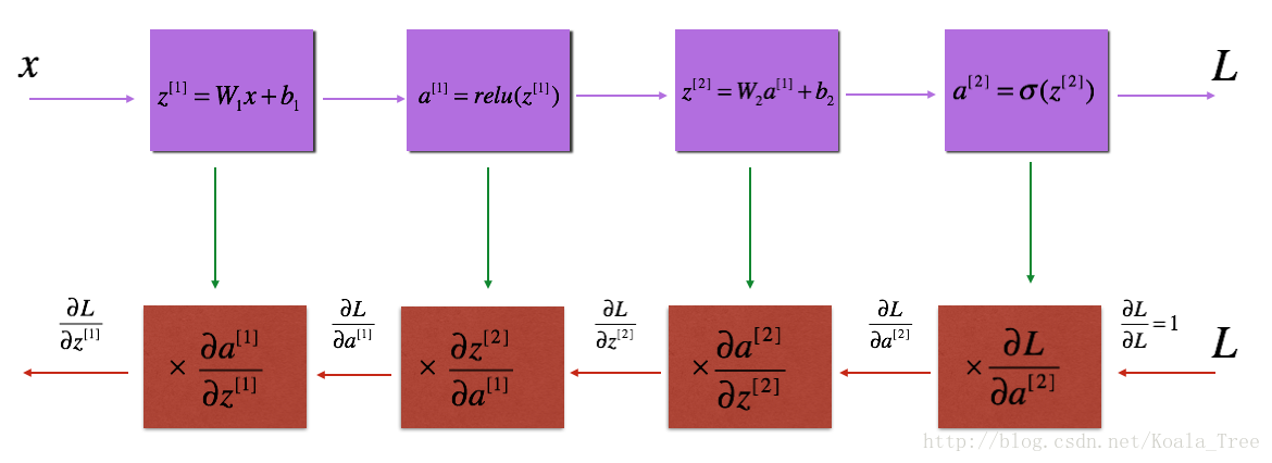
6.1 - Linear backward

对于第l层：线性的部分是： $Z^{[l]} = W^{[l]} A^{[l-1]} + b^{[l]}$ （然后是激活）

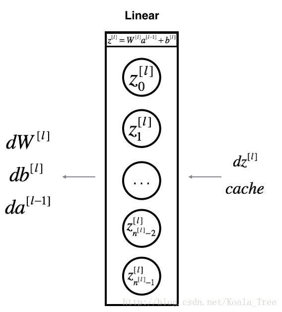
假设你已经计算过导数了 $dZ^{[l]} = \frac{\partial \mathcal{L} }{\partial Z^{[l]}}$ ，你想要得到 $(dW^{[l]}, db^{[l]} dA^{[l-1]})$

还在路上，稍等...

计算公式：

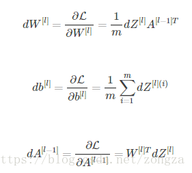
练习:使用上面的3个公式来实现下面的函数：

# GRADED FUNCTION: linear_backward

def linear_backward(dZ, cache):
    """
    Implement the linear portion of backward propagation for a single layer (layer l)

    Arguments:
    dZ -- Gradient of the cost with respect to the linear output (of current layer l)
    cache -- tuple of values (A_prev, W, b) coming from the forward propagation in the current layer

    Returns:
    dA_prev -- Gradient of the cost with respect to the activation (of the previous layer l-1), same shape as A_prev
    dW -- Gradient of the cost with respect to W (current layer l), same shape as W
    db -- Gradient of the cost with respect to b (current layer l), same shape as b
    """
    A_prev, W, b = cache
    m = A_prev.shape[1]

    ### START CODE HERE ### (≈ 3 lines of code)
    dW = np.dot(dZ, A_prev.T) / m #刚开始忘了除以m做平均
    db = np.sum(dZ, axis=1, keepdims=True) / m #刚开始没有reshape导致b的shape是（1，）,而且还没有除以m做平均
    dA_prev = np.dot(W.T, dZ)
    ### END CODE HERE ###

    assert (dA_prev.shape == A_prev.shape)
    assert (dW.shape == W.shape)
    assert (db.shape == b.shape)

    return dA_prev, dW, db

# Set up some test inputs
dZ, linear_cache = linear_backward_test_case()

dA_prev, dW, db = linear_backward(dZ, linear_cache)
print ("dA_prev = "+ str(dA_prev))
print ("dW = " + str(dW))
print ("db = " + str(db))

#linear_backward_test_case function:
def linear_backward_test_case():
    np.random.seed(1)
    dZ = np.random.randn(1,2)
    A = np.random.randn(3,2)
    W = np.random.randn(1,3)
    b = np.random.randn(1,1)
    linear_cache = (A, W, b)
    return dZ, linear_cache

dA_prev = [[ 0.51822968 -0.19517421]
 [-0.40506361  0.15255393]
 [ 2.37496825 -0.89445391]]
dW = [[-0.10076895  1.40685096  1.64992505]]
db = [[ 0.50629448]]

6.2- Linear-Activation backward

类似 Linear-Activation forward（），将 linear_backward 和 activation_backward 合并成一个函数

其中activation_backward 我们已经实现了

练习:实现线性->激活层的反向传播。

# GRADED FUNCTION: linear_activation_backward

def linear_activation_backward(dA, cache, activation):
    """
    Implement the backward propagation for the LINEAR->ACTIVATION layer.

    Arguments:
    dA -- post-activation gradient for current layer l 
    cache -- tuple of values (linear_cache, activation_cache) we store for computing backward propagation efficiently
    activation -- the activation to be used in this layer, stored as a text string: "sigmoid" or "relu"

    Returns:
    dA_prev -- Gradient of the cost with respect to the activation (of the previous layer l-1), same shape as A_prev
    dW -- Gradient of the cost with respect to W (current layer l), same shape as W
    db -- Gradient of the cost with respect to b (current layer l), same shape as b
    """
    linear_cache, activation_cache = cache

    if activation == "relu":
        ### START CODE HERE ### (≈ 2 lines of code)
        dZ = relu_backward(dA, activation_cache)
        dA_prev, dW, db = linear_backward(dZ, linear_cache)
        ### END CODE HERE ###

    elif activation == "sigmoid":
        ### START CODE HERE ### (≈ 2 lines of code)
        dZ = sigmoid_backward(dA, activation_cache)
        dA_prev, dW, db = linear_backward(dZ, linear_cache)
        ### END CODE HERE ###

    return dA_prev, dW, db

AL, linear_activation_cache = linear_activation_backward_test_case()

dA_prev, dW, db = linear_activation_backward(AL, linear_activation_cache, activation = "sigmoid")
print ("sigmoid:")
print ("dA_prev = "+ str(dA_prev))
print ("dW = " + str(dW))
print ("db = " + str(db) + "\n")

dA_prev, dW, db = linear_activation_backward(AL, linear_activation_cache, activation = "relu")
print ("relu:")
print ("dA_prev = "+ str(dA_prev))
print ("dW = " + str(dW))
print ("db = " + str(db))

#linear_activation_backward_test_case function:
def linear_activation_backward_test_case():
    np.random.seed(2)
    dA = np.random.randn(1,2)
    A = np.random.randn(3,2)
    W = np.random.randn(1,3)
    b = np.random.randn(1,1)
    Z = np.random.randn(1,2)
    linear_cache = (A, W, b)
    activation_cache = Z
    linear_activation_cache = (linear_cache, activation_cache)

    return dA, linear_activation_cache

sigmoid:
dA_prev = [[ 0.11017994  0.01105339]
 [ 0.09466817  0.00949723]
 [-0.05743092 -0.00576154]]
dW = [[ 0.10266786  0.09778551 -0.01968084]]
db = [[-0.05729622]]

relu:
dA_prev = [[ 0.44090989  0.        ]
 [ 0.37883606  0.        ]
 [-0.2298228   0.        ]]
dW = [[ 0.44513824  0.37371418 -0.10478989]]
db = [[-0.20837892]]

6.3 - L-Model Backward

拓扑：

还在路上，稍等...

正向传播：由A_l-1 和W_l,b_l 求 Z_l和A_l

反向传播：由dA_l 求 dZ_l , dW_l, db_l 和 dA_l-1

正向传播的输入就是数据X（当做A_0）而反向传播的输入（dA_L）不能直接得到，需要由cost函数计算：

dAL = - (np.divide(Y, AL) - np.divide(1 - Y, 1 - AL)) # derivative of cost with respect to AL

然后把dAL当做l_model_backward()的输入进行迭代计算各类参数的梯度，这个过程需要每一层正向传播时缓存的cache

多层神经网络拓扑：[LINEAR->RELU] ×× (L-1) -> LINEAR -> SIGMOID

def L_model_backward(AL, Y, caches):
    """
    Implement the backward propagation for the [LINEAR->RELU] * (L-1) -> LINEAR -> SIGMOID group

    Arguments:
    AL -- probability vector, output of the forward propagation (L_model_forward())
    Y -- true "label" vector (containing 0 if non-cat, 1 if cat)
    caches -- list of caches containing:
                every cache of linear_activation_forward() with "relu" (it's caches[l], for l in range(L-1) i.e l = 0...L-2)
                the cache of linear_activation_forward() with "sigmoid" (it's caches[L-1])

    Returns:
    grads -- A dictionary with the gradients
             grads["dA" + str(l)] = ...
             grads["dW" + str(l)] = ...
             grads["db" + str(l)] = ...
    """
    grads = {}
    L = len(caches)  # the number of layers
    m = AL.shape[1]
    Y = Y.reshape(AL.shape)  # after this line, Y is the same shape as AL

    # Initializing the backpropagation 激活函数的反向
    ### START CODE HERE ### (1 line of code)
    dAL = - (np.divide(Y, AL) - np.divide(1 - Y, 1 - AL)) # derivative of cost with respect to AL
    ### END CODE HERE ###

    # Lth layer (SIGMOID -> LINEAR) gradients. Inputs: "dAL, current_cache". Outputs: "grads["dAL-1"], grads["dWL"], grads["dbL"] 线性函数的反向
    ### START CODE HERE ### (approx. 2 lines)
    current_cache = caches[L-1] #L-1是因为caches用的append，所以从下标0开始的，那么第L层的缓存的下标就是L-1
    grads["dA" + str(L - 1)], grads["dW" + str(L)], grads["db" + str(L)] = linear_activation_backward(dAL,current_cache,activation="sigmoid")#注意输出的dA是上一层的和dW不是同层参数所以下标要不同
    ### END CODE HERE ###

    # Loop from l=L-2 to l=0
    for l in reversed(range(L - 1)):
        # lth layer: (RELU -> LINEAR) gradients.
        # Inputs: "grads["dA" + str(l + 1)], current_cache". Outputs: "grads["dA" + str(l)] , grads["dW" + str(l + 1)] , grads["db" + str(l + 1)]
        ### START CODE HERE ### (approx. 5 lines)
        current_cache = caches[l]
        dA_prev_temp, dW_temp, db_temp = linear_activation_backward(grads["dA"+str(l+1)],current_cache,activation="relu")
        grads["dA" + str(l)] = dA_prev_temp#这里同样注意得出的结果dA和dWdb不在同一层
        grads["dW" + str(l + 1)] = dW_temp
        grads["db" + str(l + 1)] = db_temp
        ### END CODE HERE ###


    return grads

AL, Y_assess, caches = L_model_backward_test_case()
grads = L_model_backward(AL, Y_assess, caches)
print_grads(grads)

#L_model_backward_test_case function:
def L_model_backward_test_case():
    np.random.seed(3)
    AL = np.random.randn(1, 2)
    Y = np.array([[1, 0]])

    A1 = np.random.randn(4,2)
    W1 = np.random.randn(3,4)
    b1 = np.random.randn(3,1)
    Z1 = np.random.randn(3,2)
    linear_cache_activation_1 = ((A1, W1, b1), Z1)

    A2 = np.random.randn(3,2)
    W2 = np.random.randn(1,3)
    b2 = np.random.randn(1,1)
    Z2 = np.random.randn(1,2)
    linear_cache_activation_2 = ( (A2, W2, b2), Z2)

    caches = (linear_cache_activation_1, linear_cache_activation_2)

    return AL, Y, caches

dW1 = [[ 0.41010002  0.07807203  0.13798444  0.10502167]
 [ 0.          0.          0.          0.        ]
 [ 0.05283652  0.01005865  0.01777766  0.0135308 ]]
db1 = [[-0.22007063]
 [ 0.        ]
 [-0.02835349]]
dA1 = [[ 0.12913162 -0.44014127]
 [-0.14175655  0.48317296]
 [ 0.01663708 -0.05670698]]

6.4 -更新参数

更新公式：

# GRADED FUNCTION: update_parameters

def update_parameters(parameters, grads, learning_rate):
    """
    Update parameters using gradient descent

    Arguments:
    parameters -- python dictionary containing your parameters 
    grads -- python dictionary containing your gradients, output of L_model_backward

    Returns:
    parameters -- python dictionary containing your updated parameters 
                  parameters["W" + str(l)] = ... 
                  parameters["b" + str(l)] = ...
    """

    L = len(parameters) // 2 # number of layers in the neural network

    # Update rule for each parameter. Use a for loop.
    ### START CODE HERE ### (≈ 3 lines of code)
    for l in range(L):
        parameters["W" + str(l+1)] = parameters["W" + str(l+1)] - learning_rate * grads["dW" + str(l+1)]
        parameters["b" + str(l+1)] = parameters["b" + str(l+1)] - learning_rate * grads["db" + str(l+1)]
    ### END CODE HERE ###
    return parameters

parameters, grads = update_parameters_test_case()
parameters = update_parameters(parameters, grads, 0.1)

print ("W1 = "+ str(parameters["W1"]))
print ("b1 = "+ str(parameters["b1"]))
print ("W2 = "+ str(parameters["W2"]))
print ("b2 = "+ str(parameters["b2"]))

#update_parameters_test_case function:
def update_parameters_test_case():
    np.random.seed(2)
    W1 = np.random.randn(3,4)
    b1 = np.random.randn(3,1)
    W2 = np.random.randn(1,3)
    b2 = np.random.randn(1,1)
    parameters = {"W1": W1,
                  "b1": b1,
                  "W2": W2,
                  "b2": b2}
    np.random.seed(3)
    dW1 = np.random.randn(3,4)
    db1 = np.random.randn(3,1)
    dW2 = np.random.randn(1,3)
    db2 = np.random.randn(1,1)
    grads = {"dW1": dW1,
             "db1": db1,
             "dW2": dW2,
             "db2": db2}

    return parameters, grads

W1 = [[-0.59562069 -0.09991781 -2.14584584  1.82662008]
 [-1.76569676 -0.80627147  0.51115557 -1.18258802]
 [-1.0535704  -0.86128581  0.68284052  2.20374577]]
b1 = [[-0.04659241]
 [-1.28888275]
 [ 0.53405496]]
W2 = [[-0.55569196  0.0354055   1.32964895]]
b2 = [[-0.84610769]]

7-总结

没啥好说的。

part2-用于图像分类的深度神经网络:应用

1-需要的包

import time
import numpy as np
import h5py
import matplotlib.pyplot as plt
import scipy
from PIL import Image
from scipy import ndimage
from dnn_app_utils_v2 import *

%matplotlib inline
plt.rcParams['figure.figsize'] = (5.0, 4.0) # set default size of plots
plt.rcParams['image.interpolation'] = 'nearest'
plt.rcParams['image.cmap'] = 'gray'

%load_ext autoreload
%autoreload 2

np.random.seed(1)

2-数据集

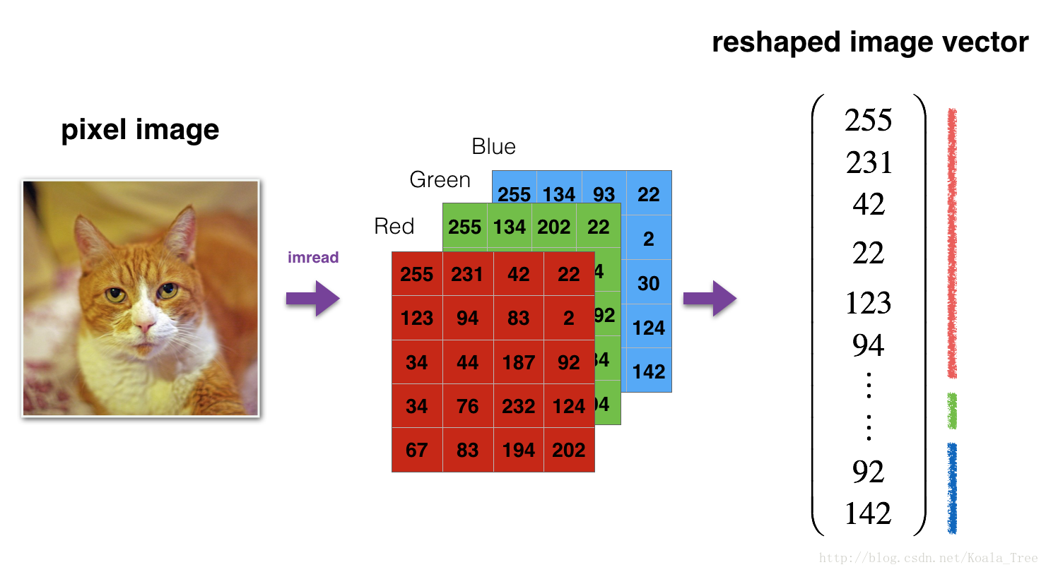
每一张图片的维度都是（num_px,num_px,3），其中3代表rgb三个通道

train_x_orig, train_y, test_x_orig, test_y, classes = load_data()

# 看看一个样例图
index = 10
plt.imshow(train_x_orig[index])
print ("y = " + str(train_y[0,index]) + ". It's a " + classes[train_y[0,index]].decode("utf-8") +  " picture.")

# 看看维度和图片数目
m_train = train_x_orig.shape[0]
num_px = train_x_orig.shape[1]
m_test = test_x_orig.shape[0]

print ("Number of training examples: " + str(m_train))
print ("Number of testing examples: " + str(m_test))
print ("Each image is of size: (" + str(num_px) + ", " + str(num_px) + ", 3)")
print ("train_x_orig shape: " + str(train_x_orig.shape))
print ("train_y shape: " + str(train_y.shape))
print ("test_x_orig shape: " + str(test_x_orig.shape))
print ("test_y shape: " + str(test_y.shape))


#在实际使用中还需要进行如下正规化处理
# Reshape the training and test examples 
train_x_flatten = train_x_orig.reshape(train_x_orig.shape[0], -1).T   # The "-1" makes reshape flatten the remaining dimensions
test_x_flatten = test_x_orig.reshape(test_x_orig.shape[0], -1).T

# Standardize data to have feature values between 0 and 1.
train_x = train_x_flatten/255.
test_x = test_x_flatten/255.

print ("train_x's shape: " + str(train_x.shape))
print ("test_x's shape: " + str(test_x.shape))

y = 0. It's a non-cat picture.

Number of training examples: 209
Number of testing examples: 50
Each image is of size: (64, 64, 3)
train_x_orig shape: (209, 64, 64, 3)
train_y shape: (1, 209)
test_x_orig shape: (50, 64, 64, 3)
test_y shape: (1, 50)

train_x's shape: (12288, 209)
test_x's shape: (12288, 50)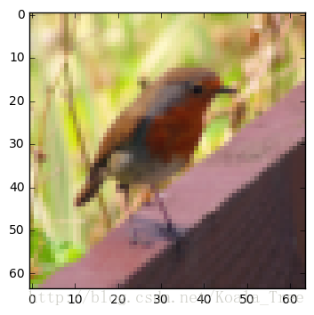

还在路上，稍等...

正规化处理：在将图像发送到网络之前，需要对其进行重新格式化和标准化。（64,64,3）reshape成一个vector后就是（12288，1）

还在路上，稍等...

3-模型

3.1两层网络

拓扑：

还在路上，稍等...

3.2 L层网络

拓扑：

还在路上，稍等...

和往常一样，您将遵循深度学习方法来构建模型:
1.初始化参数/定义超参数
2.num_iterations循环:

a.向前传播。
b.计算成本函数
c.反向传播
d.更新参数(使用参数，后支柱的梯度)

4使用经过训练的参数来预测标签

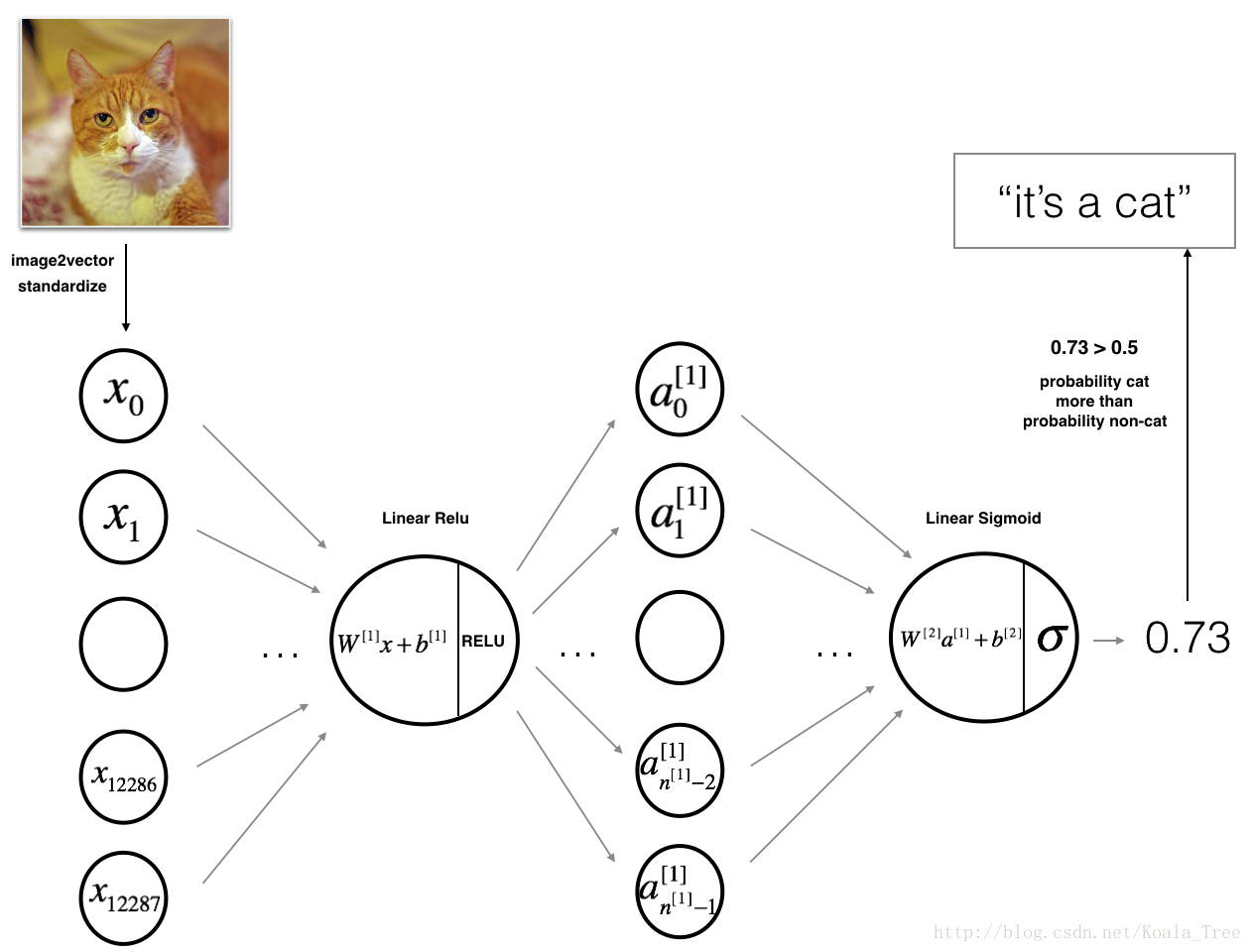
4-两层网络

拓扑：LINEAR -> RELU -> LINEAR -> SIGMOID

用到的函数：

def initialize_parameters(n_x, n_h, n_y):
    ...
    return parameters 
def linear_activation_forward(A_prev, W, b, activation):
    ...
    return A, cache
def compute_cost(AL, Y):
    ...
    return cost
def linear_activation_backward(dA, cache, activation):
    ...
    return dA_prev, dW, db
def update_parameters(parameters, grads, learning_rate):
    ...
    return parameters


### CONSTANTS DEFINING THE MODEL ####
n_x = 12288     # num_px * num_px * 3
n_h = 7
n_y = 1
layers_dims = (n_x, n_h, n_y)

代码实现：

# GRADED FUNCTION: two_layer_model

def two_layer_model(X, Y, layers_dims, learning_rate = 0.0075, num_iterations = 3000, print_cost=False):
    """
    Implements a two-layer neural network: LINEAR->RELU->LINEAR->SIGMOID.

    Arguments:
    X -- input data, of shape (n_x, number of examples)
    Y -- true "label" vector (containing 0 if cat, 1 if non-cat), of shape (1, number of examples)
    layers_dims -- dimensions of the layers (n_x, n_h, n_y)
    num_iterations -- number of iterations of the optimization loop
    learning_rate -- learning rate of the gradient descent update rule
    print_cost -- If set to True, this will print the cost every 100 iterations 

    Returns:
    parameters -- a dictionary containing W1, W2, b1, and b2
    """

    np.random.seed(1)
    grads = {}
    costs = []                              # to keep track of the cost
    m = X.shape[1]                           # number of examples
    (n_x, n_h, n_y) = layers_dims

    # Initialize parameters dictionary, by calling one of the functions you'd previously implemented
    ### START CODE HERE ### (≈ 1 line of code)
    parameters = initialize_parameters(n_x, n_h, n_y)
    ### END CODE HERE ###

    # Get W1, b1, W2 and b2 from the dictionary parameters.
    W1 = parameters["W1"]
    b1 = parameters["b1"]
    W2 = parameters["W2"]
    b2 = parameters["b2"]

    # Loop (gradient descent)

    for i in range(0, num_iterations):

        # Forward propagation: LINEAR -> RELU -> LINEAR -> SIGMOID. Inputs: "X, W1, b1". Output: "A1, cache1, A2, cache2".
        ### START CODE HERE ### (≈ 2 lines of code)
        A1, cache1 = linear_activation_forward(X, W1, b1, activation="relu")
        A2, cache2 = linear_activation_forward(A1, W2, b2, activation="sigmoid")
        ### END CODE HERE ###

        # Compute cost
        ### START CODE HERE ### (≈ 1 line of code)
        cost = compute_cost(A2, Y)
        ### END CODE HERE ###

        # Initializing backward propagation
        dA2 = - (np.divide(Y, A2) - np.divide(1 - Y, 1 - A2))

        # Backward propagation. Inputs: "dA2, cache2, cache1". Outputs: "dA1, dW2, db2; also dA0 (not used), dW1, db1".
        ### START CODE HERE ### (≈ 2 lines of code)
        dA1, dW2, db2 = linear_activation_backward(dA2, cache2, activation="sigmoid")
        dA0, dW1, db1 = linear_activation_backward(dA1, cache1, activation="relu")
        ### END CODE HERE ###

        # Set grads['dWl'] to dW1, grads['db1'] to db1, grads['dW2'] to dW2, grads['db2'] to db2
        grads['dW1'] = dW1
        grads['db1'] = db1
        grads['dW2'] = dW2
        grads['db2'] = db2

        # Update parameters.
        ### START CODE HERE ### (approx. 1 line of code)
        parameters = update_parameters(parameters, grads, learning_rate)
        ### END CODE HERE ###

        # Retrieve W1, b1, W2, b2 from parameters
        W1 = parameters["W1"]
        b1 = parameters["b1"]
        W2 = parameters["W2"]
        b2 = parameters["b2"]

        # Print the cost every 100 training example
        if print_cost and i % 100 == 0:
            print("Cost after iteration {}: {}".format(i, np.squeeze(cost)))
        if print_cost and i % 100 == 0:
            costs.append(cost)

    # plot the cost

    plt.plot(np.squeeze(costs))
    plt.ylabel('cost')
    plt.xlabel('iterations (per tens)')
    plt.title("Learning rate =" + str(learning_rate))
    plt.show()

    return parameters

查看结果：

parameters = two_layer_model(train_x, train_y, layers_dims = (n_x, n_h, n_y), num_iterations = 2500, print_cost=True)

predictions_train = predict(train_x, train_y, parameters)

predictions_test = predict(test_x, test_y, parameters)

#predict函数
def predict(X, y, parameters):
    """
    This function is used to predict the results of a  L-layer neural network.

    Arguments:
    X -- data set of examples you would like to label
    parameters -- parameters of the trained model

    Returns:
    p -- predictions for the given dataset X
    """

    m = X.shape[1]
    n = len(parameters) // 2 # number of layers in the neural network
    p = np.zeros((1,m))

    # Forward propagation
    probas, caches = L_model_forward(X, parameters)


    # convert probas to 0/1 predictions
    for i in range(0, probas.shape[1]):
        if probas[0,i] > 0.5:
            p[0,i] = 1
        else:
            p[0,i] = 0

    print("Accuracy: "  + str(np.sum((p == y)/m)))

    return p

Cost after iteration 0: 0.693049735659989
Cost after iteration 100: 0.6464320953428849
Cost after iteration 200: 0.6325140647912678
Cost after iteration 300: 0.6015024920354665
Cost after iteration 400: 0.5601966311605748
Cost after iteration 500: 0.515830477276473
Cost after iteration 600: 0.4754901313943325
Cost after iteration 700: 0.43391631512257495
Cost after iteration 800: 0.4007977536203886
Cost after iteration 900: 0.35807050113237987
Cost after iteration 1000: 0.3394281538366413
Cost after iteration 1100: 0.30527536361962654
Cost after iteration 1200: 0.2749137728213015
Cost after iteration 1300: 0.24681768210614827
Cost after iteration 1400: 0.1985073503746611
Cost after iteration 1500: 0.17448318112556593
Cost after iteration 1600: 0.1708076297809661
Cost after iteration 1700: 0.11306524562164737
Cost after iteration 1800: 0.09629426845937163
Cost after iteration 1900: 0.08342617959726878
Cost after iteration 2000: 0.0743907870431909
Cost after iteration 2100: 0.06630748132267938
Cost after iteration 2200: 0.05919329501038176
Cost after iteration 2300: 0.05336140348560564
Cost after iteration 2400: 0.048554785628770226

Accuracy: 1.0
Accuracy: 0.72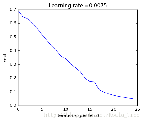

还在路上，稍等...

注意:您可能会注意到，在更少的迭代中运行模型(比如1500次)可以提高测试集的准确性。early-stopping是防止过拟合的一种方法。

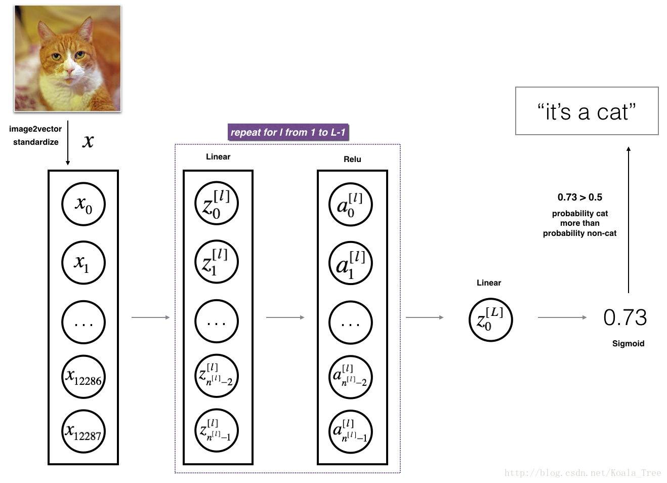
5-L层网络

拓扑：[LINEAR -> RELU]××(L-1) -> LINEAR -> SIGMOID

用到的函数：

def initialize_parameters_deep(layer_dims):
    ...
    return parameters 
def L_model_forward(X, parameters):
    ...
    return AL, caches
def compute_cost(AL, Y):
    ...
    return cost
def L_model_backward(AL, Y, caches):
    ...
    return grads
def update_parameters(parameters, grads, learning_rate):
    ...
    return parameters


### CONSTANTS ###
layers_dims = [12288, 20, 7, 5, 1] #  5-layer model

代码实现：

# GRADED FUNCTION: L_model_backward

def L_model_backward(AL, Y, caches):
    """
    Implement the backward propagation for the [LINEAR->RELU] * (L-1) -> LINEAR -> SIGMOID group

    Arguments:
    AL -- probability vector, output of the forward propagation (L_model_forward())
    Y -- true "label" vector (containing 0 if non-cat, 1 if cat)
    caches -- list of caches containing:
                every cache of linear_activation_forward() with "relu" (it's caches[l], for l in range(L-1) i.e l = 0...L-2)
                the cache of linear_activation_forward() with "sigmoid" (it's caches[L-1])

    Returns:
    grads -- A dictionary with the gradients
             grads["dA" + str(l)] = ... 
             grads["dW" + str(l)] = ...
             grads["db" + str(l)] = ... 
    """
    grads = {}
    L = len(caches) # the number of layers
    m = AL.shape[1]
    Y = Y.reshape(AL.shape) # after this line, Y is the same shape as AL

    # Initializing the backpropagation
    ### START CODE HERE ### (1 line of code)
    dAL = - (np.divide(Y, AL) - np.divide(1 - Y, 1 - AL))
    ### END CODE HERE ###

    # Lth layer (SIGMOID -> LINEAR) gradients. Inputs: "AL, Y, caches". Outputs: "grads["dAL"], grads["dWL"], grads["dbL"]
    ### START CODE HERE ### (approx. 2 lines)
    current_cache = caches[L-1]
    grads["dA" + str(L)], grads["dW" + str(L)], grads["db" + str(L)] = linear_activation_backward(dAL, current_cache, "sigmoid")
    ### END CODE HERE ###

    for l in reversed(range(L-1)):
        # lth layer: (RELU -> LINEAR) gradients.
        # Inputs: "grads["dA" + str(l + 2)], caches". Outputs: "grads["dA" + str(l + 1)] , grads["dW" + str(l + 1)] , grads["db" + str(l + 1)] 
        ### START CODE HERE ### (approx. 5 lines)
        current_cache = caches[l]
        dA_prev_temp, dW_temp, db_temp = linear_activation_backward(grads["dA" + str(l + 2)], current_cache, "relu")
        grads["dA" + str(l + 1)] = dA_prev_temp
        grads["dW" + str(l + 1)] = dW_temp
        grads["db" + str(l + 1)] = db_temp
        ### END CODE HERE ###

    return grads

查看结果：

parameters = L_layer_model(train_x, train_y, layers_dims, num_iterations = 2500, print_cost = True)

pred_train = predict(train_x, train_y, parameters)

pred_test = predict(test_x, test_y, parameters)

Cost after iteration 0: 0.771749
Cost after iteration 100: 0.672053
Cost after iteration 200: 0.648263
Cost after iteration 300: 0.611507
Cost after iteration 400: 0.567047
Cost after iteration 500: 0.540138
Cost after iteration 600: 0.527930
Cost after iteration 700: 0.465477
Cost after iteration 800: 0.369126
Cost after iteration 900: 0.391747
Cost after iteration 1000: 0.315187
Cost after iteration 1100: 0.272700
Cost after iteration 1200: 0.237419
Cost after iteration 1300: 0.199601
Cost after iteration 1400: 0.189263
Cost after iteration 1500: 0.161189
Cost after iteration 1600: 0.148214
Cost after iteration 1700: 0.137775
Cost after iteration 1800: 0.129740
Cost after iteration 1900: 0.121225
Cost after iteration 2000: 0.113821
Cost after iteration 2100: 0.107839
Cost after iteration 2200: 0.102855
Cost after iteration 2300: 0.100897
Cost after iteration 2400: 0.092878


Accuracy: 0.985645933014
Accuracy: 0.8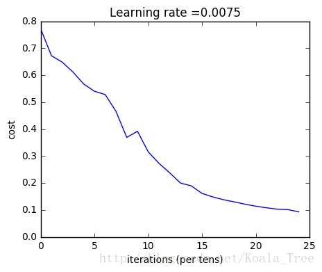

还在路上，稍等...

6-结果分析

查看预测错误的图：

print_mislabeled_images(classes, test_x, test_y, pred_test)

#具体函数：
def print_mislabeled_images(classes, X, y, p):
    """
    Plots images where predictions and truth were different.
    X -- dataset
    y -- true labels
    p -- predictions
    """
    a = p + y
    mislabeled_indices = np.asarray(np.where(a == 1))
    plt.rcParams['figure.figsize'] = (40.0, 40.0) # set default size of plots
    num_images = len(mislabeled_indices[0])
    for i in range(num_images):
        index = mislabeled_indices[1][i]
        
        plt.subplot(2, num_images, i + 1)
        plt.imshow(X[:,index].reshape(64,64,3), interpolation='nearest')
        plt.axis('off')
        plt.title("Prediction: " + classes[int(p[0,index])].decode("utf-8") + " \n Class: " + classes[y[0,index]].decode("utf-8"))
        plt.show()#这里刚开始ng没加，导致没有图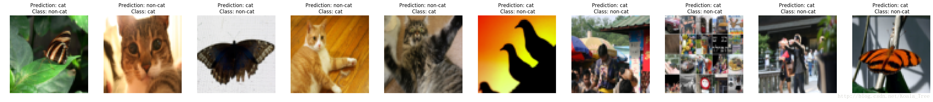

还在路上，稍等...

错误原因：

-猫的身体在一个不寻常的位置
-猫出现在一个类似的背景颜色
-不同寻常的猫的颜色和种类
-相机角度
-图片的亮度
-尺度变化(cat在图像上非常大或很小)

吴恩达Coursera深度学习课程 course1-week4 深层神经网络作业

P0 前言

P1 作业

Part-1 ：逐步建立你的深层神经网络

1-Packages

2-作业大纲

3-初始化

4-正向传播模型

5- 损失函数

6-后向传播模型

7-总结

part2-用于图像分类的深度神经网络:应用

1-需要的包

2-数据集

3-模型

4-两层网络

5-L层网络

6-结果分析

猜你喜欢

吴恩达Coursera深度学习课程 course1-week4 深层神经网络 作业

P0 前言

P1 作业

Part-1 ：逐步建立你的深层神经网络

1-Packages

2-作业大纲

3-初始化

4-正向传播模型

5- 损失函数

6-后向传播模型

7-总结

part2-用于图像分类的深度神经网络:应用

1-需要的包

2-数据集

3-模型

4-两层网络

5-L层网络

6-结果分析

猜你喜欢

吴恩达Coursera深度学习课程 course1-week4 深层神经网络作业