神经网络基础:
本篇以最简单的多个输入一个输出的1层神经网络为例,使用logistic regression讲解了神经网络的前向反向计算(forward/backward propagation)、损失和成本函数(loss/cost function)、梯度下降(gradient)和向量化(vectorization)。
一、二分分类(binary classification)
In a binary classification problem, the result is a discrete value output (1 or 0).
Example: Cat vs Non-Cat
The goal is to train a classifier that the input is an image represented by a feature vector and predicts whether the corresponding label y is 1 or 0. In this case, whether this is a cat image (1) or a non-cat image (0).
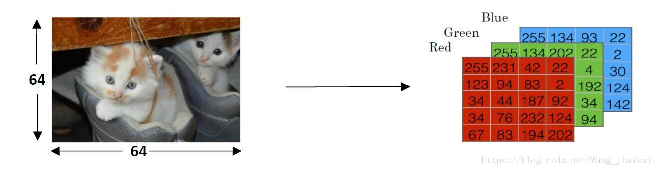
An image is store in the computer in three separate matrices corresponding to the Red, Green, and Blue color channels of the image. The three matrices have the same size as the image, for example, the resolution of the cat image is 64 pixels X 64 pixels, the three matrices (RGB) are 64 X 64 each.
The value in a cell represents the pixel intensity which will be used to create a feature vector of n dimension. In pattern recognition and machine learning, a feature vector represents an object, in this case, a cat or no cat.
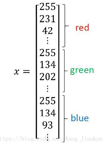
To create a feature vector, x, the pixel intensity values will be “unroll” or “reshape” for each color. The dimension of the input feature vector is nx= 64x64x3 = 12288.
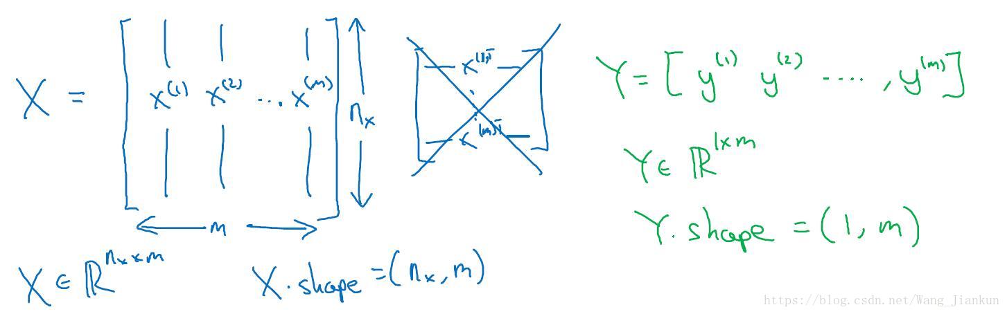
本文使用的Notation:
单个样本example:(x,y)
训练样本个数:m
每个样本的特征数:nx
所有样本:每个样本一列。X.Shape=(nx,m); Y.shape=(1,m)
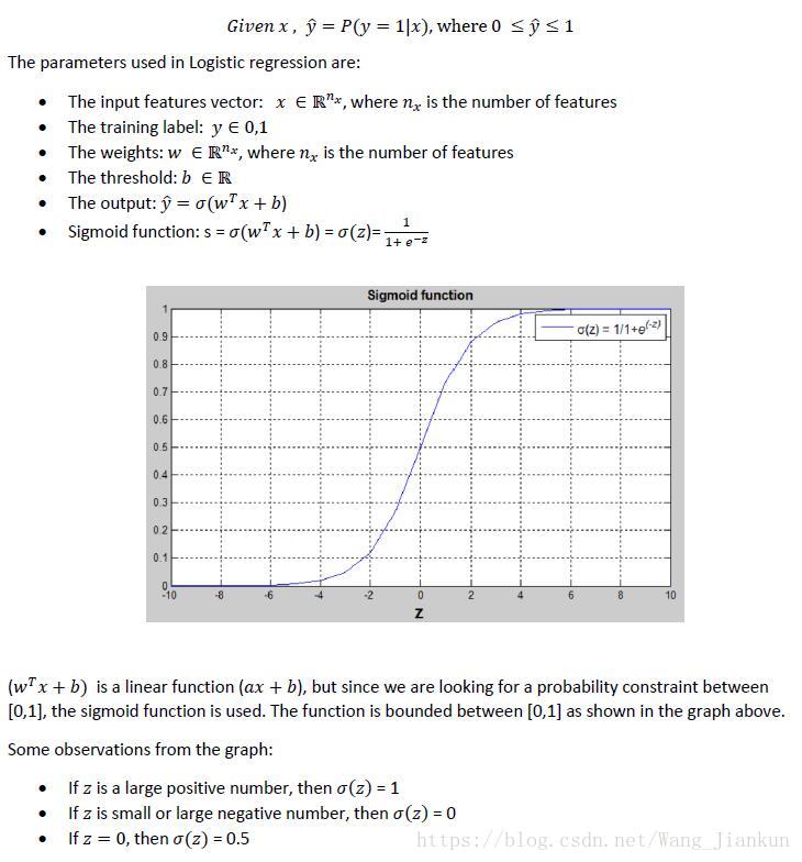
二、逻辑回归(logistic regression)
Logistic regression is a learning algorithm used in a supervised learning problem when the output y are all either zero or one. The goal of logistic regression is to minimize the error between its predictions and training data.
Given an image represented by a feature vector x, the algorithm will evaluate the probability of a cat being in that image.
三、逻辑回归损失函数(logistic regression cost function)
凸函数(convex):只有一个 local optimal solution 找到的 optimal solution 即 global optimal solution
非凸函(non-convex):有很多个 local optimal solution 找到的 optimal solution 不一定是 global optimal solution
L=(y^-y)^2是非凸函数,本文使用的L是凸函数。
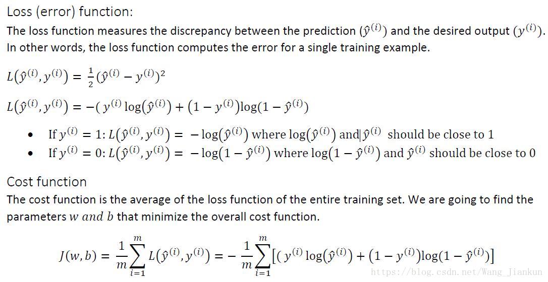
i:代表第i个example
四、梯度下降(gradient descent)
梯度下降法是用来求Cost function的最小值,经过多次迭代得到w和b的值。下图说明迭代是如何下降到 global optimal solution.
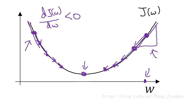
每次迭代都要更新w和b:α表示学习率(learning rate)
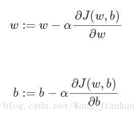
在程序中,偏导的符号通常使用dw和db来表示。
五、导数(derivatives)
只要学过点微积分的就知道什么是导数了。可以简单看做是斜率(slope)。
六、计算图(computation graph)–前向和反向传播的简单示例
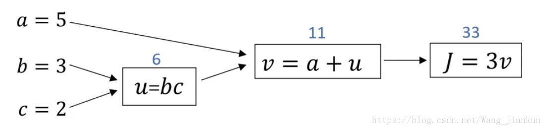
前向如上图,反向计算如下:
because: dJ/dv=3, dv/da=1, dv/du=1, du/db=c=2, du/dc=b=3
so: da=dJ/dv*dv/da=3*1=3
db=dJ/dv*dv/du*du/db=3*1*2=6
dc=dJ/dv*dv/du*du/dc=3*1*3=9
计算偏导用链式法则(chain rule)。
七、逻辑回归的梯度下降(logistic regression gradient descent )
single example:
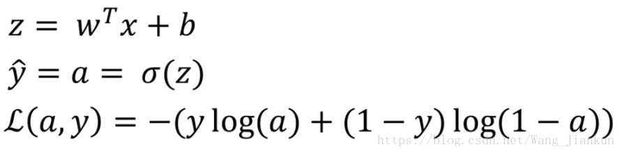
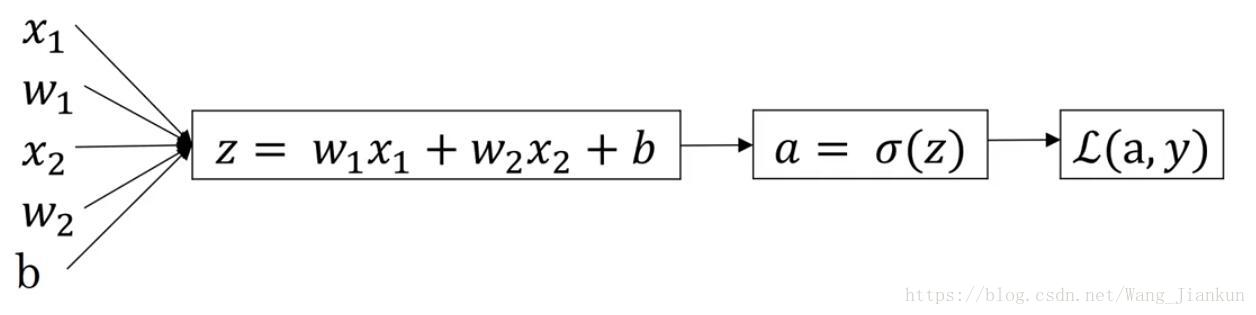
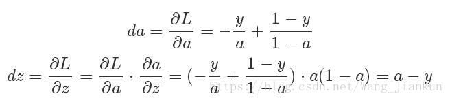
求da,dz:
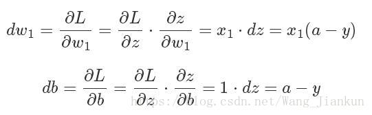
求dw1,dw2,db:
更新w和b:

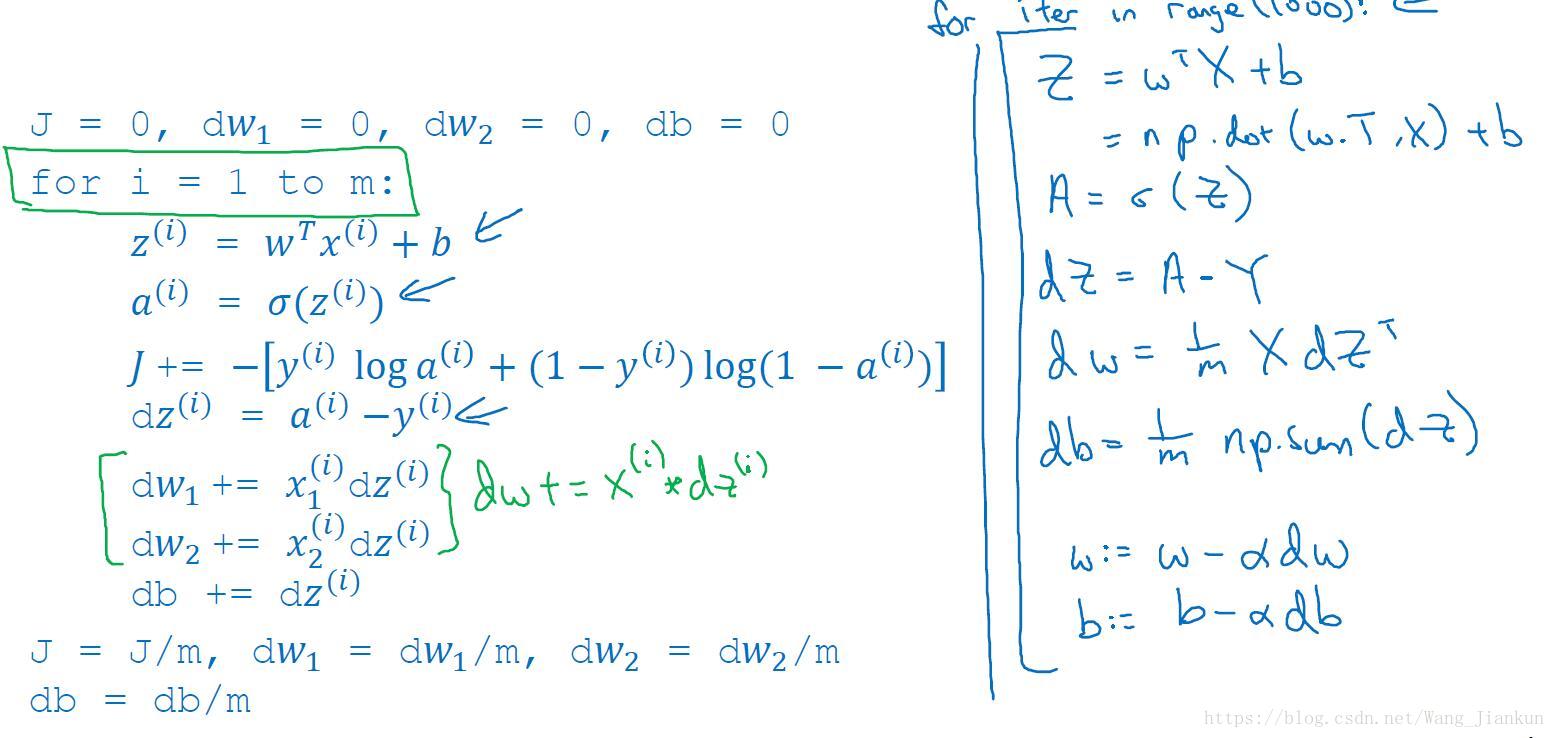
m example: 改为对cost function求导。

八、向量化(vectorization)
for loop的运行时间是向量化的几百倍,训练时通常有大量的数据所以应该尽最可能的少使用 for loop语句,利用python的numpy可以实现向量化即矩阵运算,提高程序的运行速度。
X: (nx,m) Y: (1,m) w: (nx,1) b: scalar
python代码:
Z = np.dot(w.T,X) + b
A = sigmoid(Z)
dz = A-Y
db = 1/m*np.sum(dZ)
dw = 1/m*np.dot(X,dZ.T)
w = w - alpha*dw
b = b - alpha*db
九、python的broadcasting和编程注意点
broadcasting:
矩阵加减乘除向量/数:该向量/数会自动扩展成和矩阵一样大小的矩阵
向量加减乘除数:该数会自动扩展成和向量一样大小的向量
cal = A.sum(axis=0)   #axis=0垂直相加变成行向量,=1水平相加变成列向量
A/=cal   # cal自动进行broadcasting
编程note:
#生成5个高斯随机数
a = np.random.randn(5) #rank为1,维度为(5,)
#如果需要定义(5,1)或者(1,5)向量,要使用下面标准的语句:
a = np.random.randn(5,1)
b = np.random.randn(1,5)
#使用assert语句对向量或数组的维度进行判断。不符合条件,则程序在此处停止。帮助我们及时检查、发现语句是否正确。
assert(a.shape == (5,1))
#使用reshape函数把数组设置为我们所需的维度
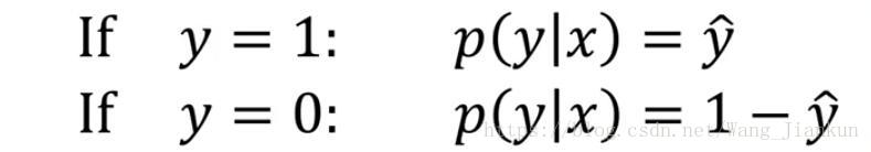
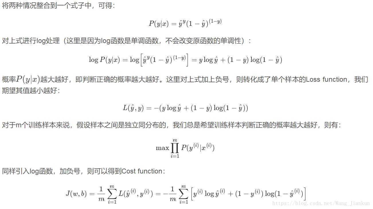
a.reshape((5,1))十、logistic loss和cost函数的理解