P0 前言

第四门课 : Convolutional Neural Networks (卷积神经网络)
第一周 : Foundations of Convolutional Neural Networks (卷积神经网络基础)
主要知识点 : 计算机视觉、边缘检测、卷积神经网络、Padding、卷积、池化等；

视频地址：https://mooc.study.163.com/learn/2001281004?tid=2001392030#/learn/content

笔记地址：以后补

数据集，源码，作业的本地版网页缓存下载：

P1 作业

Part 1：神经网络的底层搭建（Convolutional Neural Networks: Step by Step）

这里，我们要实现一个拥有卷积层（CONV）和池化层（POOL）的网络，它包含了前向和反向传播。我们来定义一下符号：

1 导入库

import numpy as np
import h5py
import matplotlib.pyplot as plt

%matplotlib inline
plt.rcParams['figure.figsize'] = (5.0, 4.0) # set default size of plots
plt.rcParams['image.interpolation'] = 'nearest'
plt.rcParams['image.cmap'] = 'gray'

%load_ext autoreload
%autoreload 2

np.random.seed(1)

2 作业大纲

我们将实现一个卷积神经网络的一些模块，下面我们将列举我们要实现的模块的函数功能：

卷积模块，包含了以下函数：

使用0扩充边界
卷积窗口
前向卷积
反向卷积（可选）

池化模块，包含了以下函数：

前向池化
创建掩码
值分配
反向池化（可选）

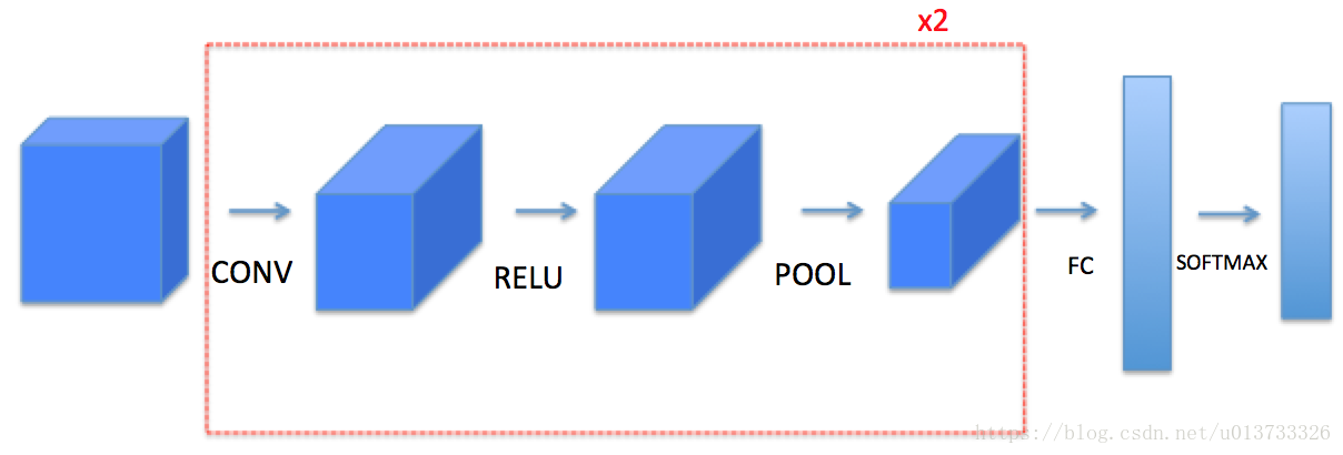
我们将在这里从底层搭建一个完整的模块，之后我们会用TensorFlow实现。模型结构如下：

需要注意的是我们在前向传播的过程中，我们会存储一些值，以便在反向传播的过程中计算梯度值。

3- 卷积神经网络

尽管编程框架使卷积容易使用，但它们仍然是深度学习中最难理解的概念之一。卷积层将输入转换成不同维度的输出，如下所示。

conv_nn

我们将一步步构建卷积层，我们将首先实现两个辅助函数：一个用于零填充，另一个用于计算卷积。

3.1 - 边界填充

边界填充将会在图像边界周围添加值为0的像素点，如下图所示：

PAD

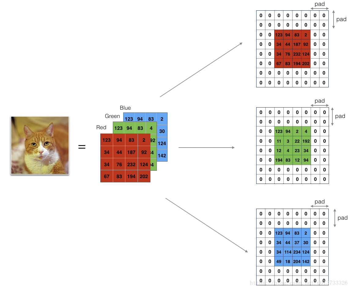
上图是使用了使用pading为2的操作对图像（3通道，RGB）进行填充。

使用0填充边界有以下好处：

帮助我们保留更多的图像边界信息。在没有填充的情况下，卷积过程中图像边缘的极少数值会受到过滤器的影响从而导致信息丢失。

使我们避免在接下来的CONV层中缩小卷积核的高度和宽度，（后面的没看懂什么意思。）（原文：It allows you to use a CONV layer without necessarily shrinking the height and width of the volumes. This is important for building deeper networks, since otherwise the height/width would shrink as you go to deeper layers. An important special case is the "same" convolution, in which the height/width is exactly preserved after one layer.）

我们将实现一个边界填充函数，它会把所有的样本图像XX都使用0进行填充。我们可以使用np.pad来快速填充。需要注意的是如果你想使用pad = 1填充数组a.shape = (5,5,5,5,5)的第二维，使用pad = 3填充第4维，使用pad = 0来填充剩下的部分，我们可以这么做：

#constant连续一样的值填充，有constant_values=（x, y）时前面用x填充，后面用y填充。缺省参数是为constant_values=（0,0）

a = np.pad(a,( (0,0),(1,1),(0,0),(3,3),(0,0)),'constant',constant_values = (..,..))

#比如：
import numpy as np
arr3D = np.array([[[1, 1, 2, 2, 3, 4],
             [1, 1, 2, 2, 3, 4], 
             [1, 1, 2, 2, 3, 4]], 

            [[0, 1, 2, 3, 4, 5], 
             [0, 1, 2, 3, 4, 5], 
             [0, 1, 2, 3, 4, 5]], 

            [[1, 1, 2, 2, 3, 4], 
             [1, 1, 2, 2, 3, 4], 
             [1, 1, 2, 2, 3, 4]]])

print 'constant:  \n' + str(np.pad(arr3D, ((0, 0), (1, 1), (2, 2)), 'constant'))
#（1,1）代表第二维填充上下各一行（2，2）代表第三维填充左右各两列

"""
constant:  
[[[0 0 0 0 0 0 0 0 0 0]
  [0 0 1 1 2 2 3 4 0 0]
  [0 0 1 1 2 2 3 4 0 0]
  [0 0 1 1 2 2 3 4 0 0]
  [0 0 0 0 0 0 0 0 0 0]]

 [[0 0 0 0 0 0 0 0 0 0]
  [0 0 0 1 2 3 4 5 0 0]
  [0 0 0 1 2 3 4 5 0 0]
  [0 0 0 1 2 3 4 5 0 0]
  [0 0 0 0 0 0 0 0 0 0]]

 [[0 0 0 0 0 0 0 0 0 0]
  [0 0 1 1 2 2 3 4 0 0]
  [0 0 1 1 2 2 3 4 0 0]
  [0 0 1 1 2 2 3 4 0 0]
  [0 0 0 0 0 0 0 0 0 0]]]
"""

0填充函数：

# GRADED FUNCTION: zero_pad

def zero_pad(X, pad):
    """
    Pad with zeros all images of the dataset X. The padding is applied to the height and width of an image,
    as illustrated in Figure 1.

    Argument:
    X -- python numpy array of shape (m, n_H, n_W, n_C) representing a batch of m images
    pad -- integer, amount of padding around each image on vertical and horizontal dimensions

    Returns:
    X_pad -- padded image of shape (m, n_H + 2*pad, n_W + 2*pad, n_C)
    """

    ### START CODE HERE ### (≈ 1 line)
    X_pad = np.pad(X,((0,0),(pad,pad),(pad,pad),(0,0)),'constant')
    #刚开始用的(0,0),(0,2*pad),(0,2*pad),(0,0)，实际上(x,y)是指左边填充x行右边y行（对应第三维）或者上边填充x行下边y行（对应第二维）
    ### END CODE HERE ###

    return X_pad

#查看结果：
    np.random.seed(1)
    x = np.random.randn(4, 3, 3, 2)
    x_pad = zero_pad(x, 2)
    print("x.shape =", x.shape)
    print("x_pad.shape =", x_pad.shape)
    print("x[1,1] =", x[1, 1])
    print("x_pad[1,1] =", x_pad[1, 1])

    fig, axarr = plt.subplots(1, 2)
    axarr[0].set_title('x')
    axarr[0].imshow(x[0, :, :, 0])
    axarr[1].set_title('x_pad')
    axarr[1].imshow(x_pad[0, :, :, 0])
    plt.show()
#结果：
x.shape = (4, 3, 3, 2)
x_pad.shape = (4, 7, 7, 2)
x[1,1] = [[ 0.90085595 -0.68372786]
 [-0.12289023 -0.93576943]
 [-0.26788808  0.53035547]]
x_pad[1,1] = [[0. 0.]
 [0. 0.]
 [0. 0.]
 [0. 0.]
 [0. 0.]
 [0. 0.]
 [0. 0.]]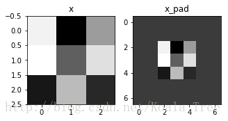

还在路上，稍等...

3.2 - Single step of convolution（单步卷积）

在这里，我们要实现第一步卷积，我们要使用一个过滤器来卷积输入的数据。先来看看下面的这个gif：

还在路上，稍等...

上图中过滤器（filter）大小：f = 2 ，步伐stride：s = 1（stride=你每次滑动时移动窗口的幅度）。

在计算机视觉应用中，左侧矩阵中的每个值都对应一个像素值，我们通过将其值与原始矩阵元素相乘，然后对它们进行求和来将3x3滤波器与图像进行卷积。我们需要实现一个函数，可以将一个3x3滤波器与单独的切片块进行卷积并输出一个实数。现在我们开始实现conv_single_step()

def conv_single_step(a_slice_prev, W, b):
    """
    Apply one filter defined by parameters W on a single slice (a_slice_prev) of the output activation
    of the previous layer.

    Arguments:
    a_slice_prev -- slice of input data of shape (f, f, n_C_prev)
    W -- Weight parameters contained in a window - matrix of shape (f, f, n_C_prev)
    b -- Bias parameters contained in a window - matrix of shape (1, 1, 1)

    Returns:
    Z -- a scalar value, result of convolving the sliding window (W, b) on a slice x of the input data
    """


    ### START CODE HERE ### (≈ 2 lines of code)
    # Element-wise product between a_slice and W. Do not add the bias yet.
    s = np.multiply(a_slice_prev,W)
    # Sum over all entries of the volume s.
    Z = np.sum(s)
    # Add bias b to Z. Cast b to a float() so that Z results in a scalar value.
    Z = Z+float(b)
    ### END CODE HERE ###

    return Z

#查看结果：
    np.random.seed(1)
    a_slice_prev = np.random.randn(4, 4, 3)
    W = np.random.randn(4, 4, 3)
    b = np.random.randn(1, 1, 1)

    Z = conv_single_step(a_slice_prev, W, b)
    print("Z =", Z)
#结果：
Z = -6.999089450680221

3.3 - Convolutional Neural Networks - Forward pass（前向传播）

在前向传播的过程中，我们将使用多种过滤器对输入的数据进行卷积操作，每个过滤器会产生一个2D的矩阵，我们可以把它们堆叠起来，于是这些2D的卷积矩阵就变成了高维的矩阵。

我们需要实现一个函数以实现对激活值进行卷积。我们需要在激活值矩阵Aprev上使用过滤器W进行卷积。该函数的输入是前一层的激活输出Aprev以及F个过滤器（其权重矩阵为W、偏置矩阵为b，每个过滤器只有一个偏置）产生。最后，我们需要一个包含了步长（stride）s和填充（padding）p的字典类型的超参数。

小提示：

如果我要在矩阵A_prev（shape = (5,5,3)）的左上角选择一个2x2的矩阵进行切片操作，那么可以这样做：

a_slice_prev = a_prev[0:2,0:2,:]

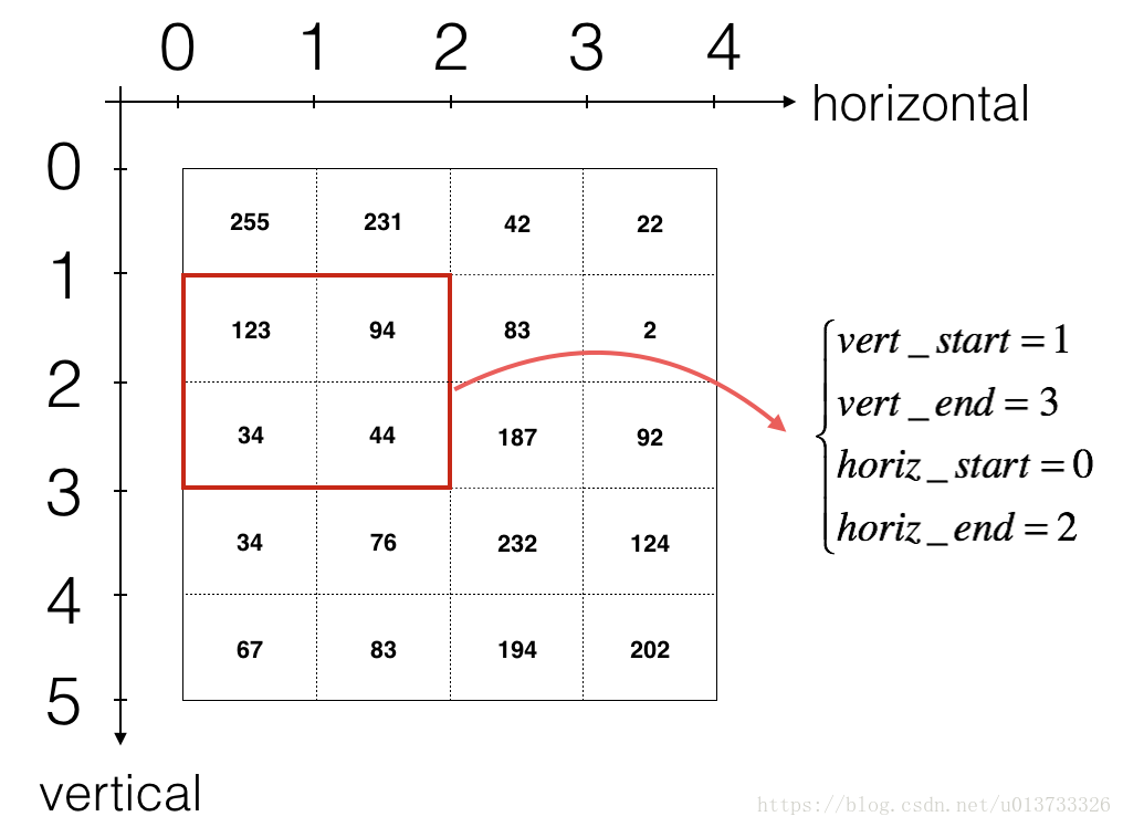
如果我想要自定义切片，我们可以这么做：先定义要切片的位置，vert_start、vert_end、 horiz_start、 horiz_end，它们的位置我们看一下下面的图（只适用于单通道）就明白了。

关于卷积的输出形状与输入形状的公式为（由输入维度计算输出维度）：

$n_H = \lfloor \frac{n_{H_{prev}} - f + 2 \times pad}{stride} \rfloor +1$

$n_W = \lfloor \frac{n_{W_{prev}} - f + 2 \times pad}{stride} \rfloor +1$

$n_C = {过滤器数量}$ 过滤器数量

这里我们不会使用矢量化，只是用for循环来实现所有的东西。

def conv_forward(A_prev, W, b, hparameters):
    """
    Implements the forward propagation for a convolution function

    Arguments:
    A_prev -- output activations of the previous layer, numpy array of shape (m, n_H_prev, n_W_prev, n_C_prev)
    W -- Weights, numpy array of shape (f, f, n_C_prev, n_C)
    b -- Biases, numpy array of shape (1, 1, 1, n_C)
    hparameters -- python dictionary containing "stride" and "pad"

    Returns:
    Z -- conv output, numpy array of shape (m, n_H, n_W, n_C)
    cache -- cache of values needed for the conv_backward() function
    """

    ### START CODE HERE ###
    # Retrieve dimensions from A_prev's shape (≈1 line)
    (m, n_H_prev, n_W_prev, n_C_prev) = A_prev.shape#n_C_prev是上一层的过滤器数量

    # Retrieve dimensions from W's shape (≈1 line)
    (f, f, n_C_prev, n_C) = ( W.shape)

    # Retrieve information from "hparameters" (≈2 lines)
    stride = hparameters["stride"]
    pad = hparameters["pad"]

    # Compute the dimensions of the CONV output volume using the formula given above. Hint: use int() to floor. (≈2 lines)
    n_H = int((n_H_prev-f+2.*pad)*1./stride)+1
    n_W = int((n_W_prev-f+2.*pad)*1./stride)+1

    # Initialize the output volume Z with zeros. (≈1 line)
    Z = np.zeros((m,n_H,n_W,n_C)) #刚开始用的Z = np.zeros((n_H,n_W))

    # Create A_prev_pad by padding A_prev
    A_prev_pad = zero_pad(A_prev,pad=pad)

    for i in range(m):  # loop over the batch of training examples
        a_prev_pad = A_prev_pad[i]  # Select ith training example's padded activation
        for h in range(n_H):  # loop over vertical axis of the output volume #刚开始用的range(n_H_prev)
            for w in range(n_W):  # loop over horizontal axis of the output volume
                for c in range(n_C):  # loop over channels (= #filters) of the output volume

                    # Find the corners of the current "slice" (≈4 lines)
                    vert_start = stride*h #刚开始用的vert_start = h
                    vert_end = vert_start+f
                    horiz_start = stride*w #刚开始使用的horiz_start = w
                    horiz_end = horiz_start+f

                    # Use the corners to define the (3D) slice of a_prev_pad (See Hint above the cell). (≈1 line)
                    a_slice_prev = a_prev_pad[vert_start:vert_end,horiz_start:horiz_end,:]#刚开似乎用的a_slice_prev = a_prev_pad[vert_start:vert_end,horiz_start:horiz_end,c]

                    # Convolve the (3D) slice with the correct filter W and bias b, to get back one output neuron. (≈1 line)
                    Z[i, h, w, c] = conv_single_step(a_slice_prev=a_slice_prev,W=W[:,:,:,c],b=b[:,:,:,c])#刚开始用的W[：，：，c，c],这里意思是说上一层的三个颜色通道（三个滤波器）全用来产生本层的一个颜色通道（一个滤波器的输出值）

    ### END CODE HERE ###

    # Making sure your output shape is correct
    assert (Z.shape == (m, n_H, n_W, n_C))

    # Save information in "cache" for the backprop
    cache = (A_prev, W, b, hparameters)

    return Z, cache

#查看结果：
    np.random.seed(1)
    A_prev = np.random.randn(10, 4, 4, 3)
    W = np.random.randn(2, 2, 3, 8)
    b = np.random.randn(1, 1, 1, 8)
    hparameters = {"pad": 2,
                   "stride": 2}

    Z, cache_conv = conv_forward(A_prev, W, b, hparameters)
    print("Z's mean =", np.mean(Z))
    print("Z[3,2,1] =", Z[3, 2, 1])
    print("b=",b[0,0,0,:])
    print("W =", W[0, 0, 0, :])
    print("cache_conv[0][1][2][3] =", cache_conv[0][1][2][3])

结果：

#结果：
Z's mean = 0.048995203528855794
Z[3,2,1] = [-0.61490741 -6.7439236  -2.55153897  1.75698377  3.56208902  0.53036437
  5.18531798  8.75898442]
b= [ 0.37245685 -0.1484898  -0.1834002   1.1010002   0.78002714 -0.6294416
 -1.1134361  -0.06741002]
W= [ 0.5154138  -1.11487105 -0.76730983  0.67457071  1.46089238  0.5924728
  1.19783084  1.70459417]
cache_conv[0][1][2][3] = [-0.20075807  0.18656139  0.41005165]

最后，卷积层应该包含一个激活函数，我们可以加一行代码来计算：

#获取输出
Z[i, h, w, c] = ...
#计算激活
A[i, h, w, c] = activation(Z[i, h, w, c])

不过，在这里我们不需要这么做。

4 - 池化层

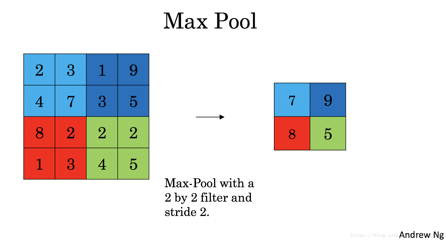
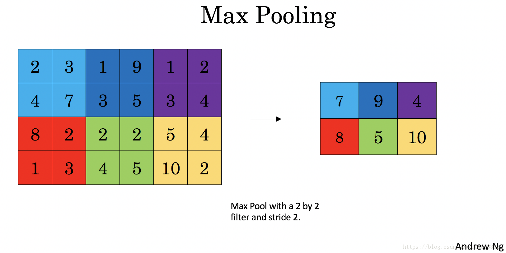
池化层会减少输入的宽度和高度，这样它会减少计算量的同时也使特征检测器对其在输入中的位置更加稳定。下面介绍两种类型的池化层：

Max-pooling layer：在输入矩阵中滑动一个大小为fxf的窗口，选取窗口里的值中的最大值，然后作为输出的一部分。

Average-pooling layer：在输入矩阵中滑动一个大小为fxf的窗口，计算窗口里的值中的平均值，然后这个均值作为输出的一部分。

池化层没有用于进行反向传播的参数，但是它们有像窗口的大小为f的超参数，它指定fxf窗口的高度和宽度，我们可以计算出最大值或平均值。

4.1 池化层的前向传播

现在我们要在同一个函数中实现最大值池化层和均值池化层。由于没有padding，池化层输出的维度和原来的维度计算公式相对简单：

$n_H = \lfloor \frac{n_{H_{prev}} - f}{stride} \rfloor +1$

$n_W = \lfloor \frac{n_{W_{prev}} - f}{stride} \rfloor +1$

$n_C = n_{C_{prev}}$

def pool_forward(A_prev, hparameters, mode="max"):
    """
    Implements the forward pass of the pooling layer

    Arguments:
    A_prev -- Input data, numpy array of shape (m, n_H_prev, n_W_prev, n_C_prev)
    hparameters -- python dictionary containing "f" and "stride"
    mode -- the pooling mode you would like to use, defined as a string ("max" or "average")

    Returns:
    A -- output of the pool layer, a numpy array of shape (m, n_H, n_W, n_C)
    cache -- cache used in the backward pass of the pooling layer, contains the input and hparameters
    """

    # Retrieve dimensions from the input shape
    (m, n_H_prev, n_W_prev, n_C_prev) = A_prev.shape

    # Retrieve hyperparameters from "hparameters"
    f = hparameters["f"]
    stride = hparameters["stride"]

    # Define the dimensions of the output
    n_H = int(1 + (n_H_prev - f) / stride)
    n_W = int(1 + (n_W_prev - f) / stride)
    n_C = n_C_prev

    # Initialize output matrix A
    A = np.zeros((m, n_H, n_W, n_C))

    ### START CODE HERE ###
    for i in range(m):  # loop over the training examples
        for h in range(n_H):  # loop on the vertical axis of the output volume
            for w in range(n_W):  # loop on the horizontal axis of the output volume
                for c in range(n_C):  # loop over the channels of the output volume

                    # Find the corners of the current "slice" (≈4 lines)
                    vert_start = stride*h
                    vert_end = vert_start+f
                    horiz_start = stride*w
                    horiz_end = horiz_start+f

                    # Use the corners to define the current slice on the ith training example of A_prev, channel c. (≈1 line)
                    a_prev_slice = A_prev[i,vert_start:vert_end,horiz_start:horiz_end,c]#这里因为没有卷积(滤波)操作所以最后一维不用全取，操作的单位是每个通道进行一次所以直接选第c个通道进行池化
                                                                                        #而卷积则是以本层层的滤波器为单位，每个滤波器进行一次操作，所以上一层的所有通道一起进行卷积

                    # Compute the pooling operation on the slice. Use an if statment to differentiate the modes. Use np.max/np.mean.
                    if mode == "max":
                        A[i, h, w, c] = np.max(a_prev_slice)
                    elif mode == "average":
                        A[i, h, w, c] = np.mean(a_prev_slice)

    ### END CODE HERE ###

    # Store the input and hparameters in "cache" for pool_backward()
    cache = (A_prev, hparameters)

    # Making sure your output shape is correct
    assert (A.shape == (m, n_H, n_W, n_C))

    return A, cache

#查看结果：    
    np.random.seed(1)
    A_prev = np.random.randn(2, 4, 4, 3)
    hparameters = {"stride": 2, "f": 3}

    A, cache = pool_forward(A_prev, hparameters)
    print("mode = max")
    print("A =", A)
    print()
    A, cache = pool_forward(A_prev, hparameters, mode="average")
    print("mode = average")
    print("A =", A)

#结果：
mode = max
A = [[[[1.74481176 0.86540763 1.13376944]]]
 [[[1.13162939 1.51981682 2.18557541]]]]

mode = average
A = [[[[ 0.02105773 -0.20328806 -0.40389855]]]
 [[[-0.22154621  0.51716526  0.48155844]]]]

5 - 卷积神经网络中的反向传播（选学）

在现在的深度学习框架中，你只需要实现前向传播，框架负责向后传播，所以大多数深度学习工程师不需要费心处理后向传播的细节，卷积网络的后向传递是有点复杂的。但是如果你愿意，你可以选择性来学习本节。

在前面的课程中，我们已经实现了一个简单的(全连接)神经网络，我们使用反向传播来计算关于更新参数的成本的梯度。类似地，在卷积神经网络中我们可以计算出关于成本的导数来更新参数。反向传播的方程并不简单，吴恩达老师并没有在课堂上推导它们，但我们可以在下面简要介绍。

5.1 - 卷积层的反向传播

我们来看一下如何实现卷积层的反向传播

5.1.1 - 计算dA

这里A_prev和W，b,Z之间的关系可以这样描述：

Z=W*A_prev+b

因此计算dA_prev时的思路是W*dZ，具体计算公式如下：

$dA += \sum ^{n_H} _{h=0} \sum ^{n_W} _{w=0} W_{c} \times dZ_{hw} \tag{1}$

其中: Z_hw = W_c * A_prev_slice + b

其中W_c是过滤器，Z_hw是当前卷积层的第h行w列的值的导数（是一个标量）。

当前卷积输出Z的每个值都相当于一个因变量，他对应的自变量是切片后的a_slice,W则相当于一个不变的系数矩阵，由于W矩阵中每个值都对计算Z有贡献(参考上面式子)，所以求dA_prev_slice时，a_slice（就是A_prev_slice，这里简写一下因为中间有一些变换，具体见代码）对应的那个W_c（不同的a_slice对应不同的W）的每个权重系数都要乘他们对应的计算结果（Z_hw）的导数。

之后把不同切片的dA_prev_slice整合起来就能得到dA_prev。

上面的解释反映到公式中就是：

da_prev_pad[vert_start:vert_end, horiz_start:horiz_end, :] += W[:,:,:,c]*dZ[i,h,w,c]
#等号左边相当于da_prev_slice
#dZ[i , h , w , c]就是由W_c和a_slice共同计算得到的一个标量
#对应当前卷积层第c个滤波器在（h，w）位置得到的滤波值

5.1.2 - 计算dW

由上面的分析可知，在求对过滤器W的导师时：可将W_c视为自变量而a_slice则作为常量。由此得出计算公式：

$dW_c += \sum^{n_H}_{h=0} \sum^{n_W}_{w=0}a_{slice} \times dZ_{hw} \tag{2}$

其中a_slice就是对应着产生了Z_hw（矩阵Z中的一个值）的那块切片，这个切片的大小是和它对应的过滤器W_c一样大的。该切片（a_slice）中每个值同样对生成Z_hw有贡献，所以求dW_c时a_slice的每个值都要乘dZ_hw。

之后把不同滤波器的dW_c整合起来就能得到某一层中所有滤波器的dW

上面解释反映到公式就是：

dW[:,:,:, c] += a_slice * dZ[i , h , w , c]
#其中等号左边就是当前卷积层第c个滤波器的参数W_c对应的导数
#dZ[i , h , w , c]就是由W_c和a_slice共同计算得到的一个标量
#对应当前卷积层第c个滤波器在（h，w）位置得到的滤波值

5.1.3 - 计算db

db计算很简单，直接上公式：

$db = \sum_{h} \sum_{w}dZ_{hw}$

和以前的神经网络一样，dbdb是由dZdZ的累加计算的，在这里，我们只需要将conv的输出ZZ的所有梯度累加就好了。在代码上我们只需要使用一行代码实现：

db[:,:,:,c] += dZ[ i, h, w, c]

5.1.4 - 函数实现

现在我们将实现反向传播函数conv_backward()，我们需要把所有的训练样本的过滤器、权值、高度、宽度都要加进来，然后使用公式1、2、3计算对应的梯度。

def conv_backward(dZ, cache):
    """
    Implement the backward propagation for a convolution function

    Arguments:
    dZ -- gradient of the cost with respect to the output of the conv layer (Z), numpy array of shape (m, n_H, n_W, n_C)
    cache -- cache of values needed for the conv_backward(), output of conv_forward()

    Returns:
    dA_prev -- gradient of the cost with respect to the input of the conv layer (A_prev),
               numpy array of shape (m, n_H_prev, n_W_prev, n_C_prev)
    dW -- gradient of the cost with respect to the weights of the conv layer (W)
          numpy array of shape (f, f, n_C_prev, n_C)
    db -- gradient of the cost with respect to the biases of the conv layer (b)
          numpy array of shape (1, 1, 1, n_C)
    """

    ### START CODE HERE ###
    # Retrieve information from "cache"
    (A_prev, W, b, hparameters) = cache

    # Retrieve dimensions from A_prev's shape
    (m, n_H_prev, n_W_prev, n_C_prev) = A_prev.shape

    # Retrieve dimensions from W's shape
    (f, f, n_C_prev, n_C) = W.shape

    # Retrieve information from "hparameters"
    stride = hparameters["stride"]
    pad = hparameters["pad"]

    # Retrieve dimensions from dZ's shape
    (m, n_H, n_W, n_C) = dZ.shape

    # Initialize dA_prev, dW, db with the correct shapes
    dA_prev = np.zeros((A_prev.shape))
    dW = np.zeros((W.shape))
    db = np.zeros((b.shape))


    # Pad A_prev and dA_prev
    A_prev_pad = zero_pad(A_prev,pad)
    dA_prev_pad = zero_pad(dA_prev,pad)

    for i in range(m):  # loop over the training examples

        # select ith training example from A_prev_pad and dA_prev_pad
        a_prev_pad = A_prev_pad[i]
        da_prev_pad = dA_prev_pad[i]

        for h in range(n_H):  # loop over vertical axis of the output volume
            for w in range(n_W):  # loop over horizontal axis of the output volume
                for c in range(n_C):  # loop over the channels of the output vo lume
                    # 刚开始用的n_C_prev，这里应该以dZ的维度为单位进行循环 (和Z的维度都一样，所以循环过程和前向传播也一样)                   

                    # Find the corners of the current "slice"
                    vert_start = stride*h
                    vert_end = vert_start+f
                    horiz_start = stride*w
                    horiz_end = horiz_start+f

                    # Use the corners to define the slice from a_prev_pad
                    a_slice = a_prev_pad[vert_start:vert_end,horiz_start:horiz_end,:]

                    # Update gradients for the window and the filter's parameters using the code formulas given above
                    da_prev_pad[vert_start:vert_end, horiz_start:horiz_end, :] += W[:,:,:,c]*dZ[i,h,w,c]#这个相当于da_prev_slice
                    dW[:, :, :, c] += a_slice*dZ[i,h,w,c]
                    db[:, :, :, c] += dZ[i,h,w,c]
                    # 其中等号左边就是当前卷积层第c个滤波器的参数W_c对应的导数
                    # dZ[i , h , w , c]就是由W_c和a_slice共同计算得到的一个标量
                    # 对应当前卷积层第c个滤波器在（h，w）位置得到的滤波值

        # Set the ith training example's dA_prev to the unpaded da_prev_pad (Hint: use X[pad:-pad, pad:-pad, :])
        dA_prev[i, :, :, :] = da_prev_pad[pad:-pad,pad:-pad,:]#这一步就是把非填充的数据取出来[pad:-pad]意思是从正数第pad行到倒数第pad行之间的数据(不包括倒数第pad行)
    ### END CODE HERE ###

    # Making sure your output shape is correct
    assert (dA_prev.shape == (m, n_H_prev, n_W_prev, n_C_prev))

    return dA_prev, dW, db

查看结果：

    np.random.seed(1)
    # 初始化参数
    A_prev = np.random.randn(10, 4, 4, 3)
    W = np.random.randn(2, 2, 3, 8)
    b = np.random.randn(1, 1, 1, 8)
    hparameters = {"pad": 2, "stride": 2}
    # 前向传播
    Z, cache_conv = conv_forward(A_prev, W, b, hparameters)
    # 后向传播
    print(Z.shape)
    #dZ = np.random.randn(10,4,4,8)
    dA, dW, db = conv_backward(Z, cache_conv)
    print("dA_mean =", np.mean(dA))
    print("dW_mean =", np.mean(dW))
    print("db_mean =", np.mean(db))

ng老师这里没给出计算dZ的方法，直接把Z当做dZ，得到的结果是：

(10, 4, 4, 8)
dA_mean = 1.45243777754
dW_mean = 1.72699145831
db_mean = 7.83923256462

5.2 - 池化层的反向传播

接下来，我们从最大值池化层开始实现池化层的反向传播。即使池化层没有反向传播过程中要更新的参数，我们仍然需要通过池化层反向传播梯度，以便为在池化层之前的层（比如卷积层）计算梯度。

5.2.1 最大值池化层的反向传播

在开始池化层的反向传播之前，我们需要创建一个create_mask_from_window()的函数，我们来看一下它是干什么的：

$X = \begin{bmatrix} 1 && 3 \\ 4 && 2 \end {bmatrix} \quad \rightarrow \quad M = \begin{bmatrix} 0 && 0 \\ 1 && 0 \end {bmatrix} \tag{4}$

正如你所看到的，这个函数创建了一个掩码矩阵，以保存最大值的位置，当为1的时候表示最大值的位置，其他的为0，这个是最大值池化层，均值池化层的向后传播也和这个差不多，但是使用的是不同的掩码。

这里先不考虑有多个最值的情况：

def create_mask_from_window(x):
    """
    Creates a mask from an input matrix x, to identify the max entry of x.

    Arguments:
    x -- Array of shape (f, f)

    Returns:
    mask -- Array of the same shape as window, contains a True at the position corresponding to the max entry of x.
    """

    ### START CODE HERE ### (≈1 line)
    mask = (x == np.max(x))
    ### END CODE HERE ###

    return mask

#查看结果：
np.random.seed(1)
x = np.random.randn(2,3)
mask = create_mask_from_window(x)
print('x = ', x)
print("mask = ", mask)
#结果
x =  [[ 1.62434536 -0.61175641 -0.52817175]
 [-1.07296862  0.86540763 -2.3015387 ]]
mask =  [[ True False False]
 [False False False]]

为什么我们要创建这一个掩码矩阵呢？想一下我们的正向传播首先是经过卷积层，然后滑动地取卷积层最大值构成了池化层，由这个最大值贡献对cost的影响，而每个影响cost的值都应该有一个非零的导数。另一个原因是：如果我们不记录最大值的位置，那么我们怎样才能反向传播到卷积层呢？

5.2.2 均值池化层的反向传播

在最大值池化层中，对于每个输入窗口，输出的所有值都来自输入中的最大值，但是在均值池化层中，因为是计算均值，所以输入窗口的每个元素对输出有一样的影响，我们来看看如何反向传播：

例如，如果我们使用2x2过滤器对前向通道进行平均池化，那么用于后向通道的掩码将如下所示:

$dZ=1 \quad \rightarrow \quad dZ = \begin{bmatrix} \frac{1}{4} && \frac{1}{4} \\ \frac{1}{4} && \frac{1}{4} \end{bmatrix}$

这意味着dZ矩阵中的每个位置对输出的贡献相等，因为在正向传递中，我们取的是平均值。

def distribute_value(dz, shape):
    """
    Distributes the input value in the matrix of dimension shape

    Arguments:
    dz -- input scalar
    shape -- the shape (n_H, n_W) of the output matrix for which we want to distribute the value of dz

    Returns:
    a -- Array of size (n_H, n_W) for which we distributed the value of dz
    """

    ### START CODE HERE ###
    # Retrieve dimensions from shape (≈1 line)
    (n_H, n_W) = shape

    # Compute the value to distribute on the matrix (≈1 line)
    average = 1.*dz/(n_H*n_W)

    # Create a matrix where every entry is the "average" value (≈1 line)
    a = np.ones(shape=shape)*average
    ### END CODE HERE ###

    return a

#查看结果：
dz = 2
shape = (2,2)
a = distribute_value(dz,shape)
print("a = " + str(a))

#结果：
a = [[ 0.5  0.5]
 [ 0.5  0.5]]

5.2.3 池化层整体的反向传播

现在您已经拥有了在池化层上计算向后传播所需的所有东西，可以着手实现整个池化层的反向传播：

def pool_backward(dA, cache, mode="max"):
    """
    Implements the backward pass of the pooling layer

    Arguments:
    dA -- gradient of cost with respect to the output of the pooling layer, same shape as A
    cache -- cache output from the forward pass of the pooling layer, contains the layer's input and hparameters
    mode -- the pooling mode you would like to use, defined as a string ("max" or "average")

    Returns:
    dA_prev -- gradient of cost with respect to the input of the pooling layer, same shape as A_prev
    """

    ### START CODE HERE ###

    # Retrieve information from cache (≈1 line)
    (A_prev, hparameters) = cache

    # Retrieve hyperparameters from "hparameters" (≈2 lines)
    stride = hparameters["stride"]
    f = hparameters["f"]

    # Retrieve dimensions from A_prev's shape and dA's shape (≈2 lines)
    m, n_H_prev, n_W_prev, n_C_prev = A_prev.shape
    m, n_H, n_W, n_C = dA.shape

    # Initialize dA_prev with zeros (≈1 line)
    dA_prev = np.zeros(A_prev.shape)

    for i in range(m):  # loop over the training examples

        # select training example from A_prev (≈1 line)
        a_prev = A_prev[i]

        for h in range(n_H):  # loop on the vertical axis
            for w in range(n_W):  # loop on the horizontal axis
                for c in range(n_C):  # loop over the channels (depth)

                    # Find the corners of the current "slice" (≈4 lines)
                    vert_start = stride*h
                    vert_end = vert_start+f
                    horiz_start = stride*w
                    horiz_end = horiz_start+f

                    # Compute the backward propagation in both modes.
                    if mode == "max":

                        # Use the corners and "c" to define the current slice from a_prev (≈1 line)
                        a_prev_slice = a_prev[vert_start:vert_end,horiz_start:horiz_end,c]
                        # Create the mask from a_prev_slice (≈1 line)
                        mask = create_mask_from_window(a_prev_slice)
                        # Set dA_prev to be dA_prev + (the mask multiplied by the correct entry of dA) (≈1 line)
                        dA_prev[i, vert_start: vert_end, horiz_start: horiz_end, c] += dA[i,h,w,c]*mask#刚开始乘的是a_prev_slice还是因为不理解原理

                    elif mode == "average":

                        # Get the value a from dA (≈1 line)
                        da = dA[i,h,w,c]
                        # Define the shape of the filter as fxf (≈1 line)
                        shape = (f,f)
                        # Distribute it to get the correct slice of dA_prev. i.e. Add the distributed value of da. (≈1 line)
                        dA_prev[i, vert_start: vert_end, horiz_start: horiz_end, c] += distribute_value(da,shape)

    ### END CODE ###

    # Making sure your output shape is correct
    assert (dA_prev.shape == A_prev.shape)

    return dA_prev

#查看结果：
    np.random.seed(1)
    A_prev = np.random.randn(5, 5, 3, 2)
    hparameters = {"stride": 1, "f": 2}
    A, cache = pool_forward(A_prev, hparameters)
    dA = np.random.randn(5, 4, 2, 2)
    dA_prev = pool_backward(dA, cache, mode="max")
    print("mode = max")
    print('mean of dA = ', np.mean(dA))
    print('dA_prev[1,1] = ', dA_prev[1, 1])
    print()
    dA_prev = pool_backward(dA, cache, mode="average")
    print("mode = average")
    print('mean of dA = ', np.mean(dA))
    print('dA_prev[1,1] = ', dA_prev[1, 1])

#结果：
mode = max
mean of dA =  0.14571390272918056
dA_prev[1,1] =  [[ 0.          0.        ]
 [ 5.05844394 -1.68282702]
 [ 0.          0.        ]]

mode = average
mean of dA =  0.14571390272918056
dA_prev[1,1] =  [[ 0.08485462  0.2787552 ]
 [ 1.26461098 -0.25749373]
 [ 1.17975636 -0.53624893]]

Part2 神经网络的应用

我们已经使用了原生代码实现了卷积神经网络，现在我们要使用TensorFlow来实现，然后应用到手势识别中，在这里我们要实现4个函数，一起来看看吧~

1 Tensorflow模型

首先导入库：

# -*- encoding:utf-8 -*-
import math
import numpy as np
import h5py
import matplotlib.pyplot as plt
import scipy
from PIL import Image
from scipy import ndimage
import tensorflow as tf
from tensorflow.python.framework import ops
from cnn_utils import *

#%matplotlib inline
np.random.seed(1)

我们使用course2 week3中的相同的手势数据集：https://blog.csdn.net/zongza/article/details/83344053

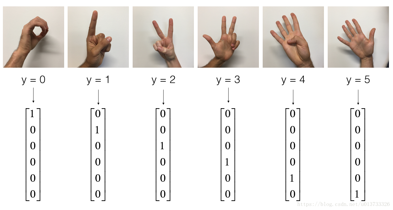
我们再来看一下里面有什么：

index = 6
plt.imshow(X_train_orig[index])
plt.show()
print ("y = " + str(np.squeeze(Y_train_orig[:, index])))

#结果：
y = 2

y=2

在course2 week3中，我们已经建立过一个神经网络，我想对这个数据集应该不陌生，我们再来看一下数据的维度，如果你忘记了独热编码的实现，可回头看这里：https://blog.csdn.net/zongza/article/details/83344053#t6

X_train = X_train_orig/255.
X_test = X_test_orig/255.
Y_train = cnn_utils.convert_to_one_hot(Y_train_orig, 6).T
Y_test = cnn_utils.convert_to_one_hot(Y_test_orig, 6).T
print ("number of training examples = " + str(X_train.shape[0]))
print ("number of test examples = " + str(X_test.shape[0]))
print ("X_train shape: " + str(X_train.shape))
print ("Y_train shape: " + str(Y_train.shape))
print ("X_test shape: " + str(X_test.shape))
print ("Y_test shape: " + str(Y_test.shape))
conv_layers = {}

#结果：
number of training examples = 1080
number of test examples = 120
X_train shape: (1080, 64, 64, 3)
Y_train shape: (1080, 6)
X_test shape: (120, 64, 64, 3)
Y_test shape: (120, 6)

1.1 创建placeholders

TensorFlow要求您为输入数据创建占位符（placeholder）真正的数据将在运行session时输入到模型中。现在我们要实现为输入X和输出Y创建占位符的函数，因为我们使用的batch_size可能不确定，所以我们在数量那里我们要使用None作为可变数量。输入X的维度为[None, n_H0, n_W0, n_C0]，对应的Y是[None, n_y]。占位符使用参考：https://www.w3cschool.cn/tensorflow_python/tensorflow_python-w7yt2fwc.html

# GRADED FUNCTION: create_placeholders

def create_placeholders(n_H0, n_W0, n_C0, n_y):
    """
    Creates the placeholders for the tensorflow session.

    Arguments:
    n_H0 -- scalar, height of an input image
    n_W0 -- scalar, width of an input image
    n_C0 -- scalar, number of channels of the input
    n_y -- scalar, number of classes

    Returns:
    X -- placeholder for the data input, of shape [None, n_H0, n_W0, n_C0] and dtype "float"
    Y -- placeholder for the input labels, of shape [None, n_y] and dtype "float"
    """


    ### START CODE HERE ### (≈2 lines)
    X = tf.placeholder(tf.float32,shape=[None,n_H0,n_W0,n_C0],name="X")
    Y = tf.placeholder(tf.float32,shape=[None,n_y],name="Y")
    ### END CODE HERE ###

    return X, Y

查看结果：

#查看结果：
X, Y = create_placeholders(64, 64, 3, 6)
print ("X = " + str(X))
print ("Y = " + str(Y))

#结果：
X = Tensor("X:0", shape=(?, 64, 64, 3), dtype=float32)
Y = Tensor("Y:0", shape=(?, 6), dtype=float32)

1.2 初始化参数

现在我们将使用tf.contrib.layers.xavier_initializer(seed = 0) 来初始化权值/过滤器W1、W2。在这里，我们不需要考虑偏置b，因为TensorFlow会考虑到的。需要注意的是我们只需要初始化2D卷积函数，全连接层TensorFlow会自动初始化的。

# GRADED FUNCTION: initialize_parameters

def initialize_parameters():
    """
    Initializes weight parameters to build a neural network with tensorflow. The shapes are:
                        W1 : [4, 4, 3, 8]
                        W2 : [2, 2, 8, 16]
    Returns:
    parameters -- a dictionary of tensors containing W1, W2
    """

    tf.set_random_seed(1)  # so that your "random" numbers match ours

    ### START CODE HERE ### (approx. 2 lines of code)
    W1 = tf.get_variable("W1", [4, 4, 3, 8], initializer=tf.contrib.layers.xavier_initializer(seed=0))
    W2 = tf.get_variable("W2", [2, 2, 8, 16], initializer=tf.contrib.layers.xavier_initializer(seed=0))
    '''
    刚开始写成：
    W1 = tf.constant(shape=[4,4,3,8],dtype=tf.float32)
    W2 = tf.constant(shape=[2,2,8,16],dtype=tf.float32)
    关于get_variable()函数：https://blog.csdn.net/u012436149/article/details/53696970/
    '''
    ### END CODE HERE ###


    parameters = {"W1": W1,
                  "W2": W2}

    return parameters

关于tf.get_variable()和tf.variable() ： https://blog.csdn.net/u012436149/article/details/53696970/

查看结果：

    tf.reset_default_graph()
    with tf.Session() as sess_test:
        parameters = initialize_parameters()
        init = tf.global_variables_initializer()
        sess_test.run(init)
        print("W1 = " + str(parameters["W1"].eval()[1, 1, 1]))
        print("W2 = " + str(parameters["W2"].eval()[1, 1, 1]))
        sess_test.close()

W1 = [ 0.00131723  0.1417614  -0.04434952  0.09197326  0.14984085 -0.03514394
 -0.06847463  0.05245192]
W2 = [-0.08566415  0.17750949  0.11974221  0.16773748 -0.0830943  -0.08058
 -0.00577033 -0.14643836  0.24162132 -0.05857408 -0.19055021  0.1345228
 -0.22779644 -0.1601823  -0.16117483 -0.10286498]

1.2 - 前向传播

在TensorFlow里面有一些可以直接拿来用的函数：

tf.nn.conv2d(X,W1,strides=[1,s,s,1],padding='SAME'):给定输入X和一组过滤器W1，这个函数将会自动使用W1来对X进行卷积，第三个输入参数是[1,s,s,1]是指对于输入 (m, n_H_prev, n_W_prev, n_C_prev)而言，每次滑动的步伐。文档参考文档参考2

tf.nn.max_pool(A, ksize = [1,f,f,1], strides = [1,s,s,1], padding = 'SAME')：给定输入X，该函数将会使用大小为（f,f）以及步伐为(s,s)的窗口对其进行滑动取最大值。参考文档

tf.nn.relu(Z1)：计算Z1的ReLU激活。参考文档

tf.contrib.layers.flatten(P)：给定一个输入P，此函数将会把每个样本转化成一维的向量，然后返回一个tensor变量，其维度为（batch_size,k）。参考文档

tf.contrib.layers.fully_connected(F, num_outputs)：给定一个已经一维化了的输入F，此函数将会返回一个由全连接层计算过后的输出。参考文档

使用tf.contrib.layers.fully_connected(F, num_outputs)的时候，全连接层会自动初始化权值且在你训练模型的时候它也会一直参与，所以当我们初始化参数的时候我们不需要专门去初始化它的权值。

我们实现前向传播的时候，我们需要定义一下我们模型的大概样子：

CONV2D -> RELU -> MAXPOOL -> CONV2D -> RELU -> MAXPOOL -> FLATTEN -> FULLYCONNECTED

我们具体实现的时候，我们需要使用以下的步骤和参数：

Conv2d : 步伐：1，填充方式：“SAME”

ReLU

Max pool : 过滤器大小：8x8，步伐：8x8，填充方式：“SAME”

Conv2d : 步伐：1，填充方式：“SAME”

ReLU

Max pool : 过滤器大小：4x4，步伐：4x4，填充方式：“SAME”

一维化上一层的输出

全连接层（FC）：使用没有非线性激活函数的全连接层。这里不要调用SoftMax，这将导致输出层中有6个神经元，然后再传递到softmax。在TensorFlow中，softmax和cost函数被集中到一个函数中，在计算成本时您将调用不同的函数。

# GRADED FUNCTION: forward_propagation

def forward_propagation(X, parameters):
    """
    Implements the forward propagation for the model:
    CONV2D -> RELU -> MAXPOOL -> CONV2D -> RELU -> MAXPOOL -> FLATTEN -> FULLYCONNECTED

    Arguments:
    X -- input dataset placeholder, of shape (input size, number of examples)
    parameters -- python dictionary containing your parameters "W1", "W2"
                  the shapes are given in initialize_parameters

    Returns:
    Z3 -- the output of the last LINEAR unit
    """

    # Retrieve the parameters from the dictionary "parameters"
    W1 = parameters['W1']
    W2 = parameters['W2']

    ### START CODE HERE ###
    '''
    #刚开始加加了这两句，但是实际上s和f的值下面注释中有提示
    s = parameters["stride"]
    f = parameters["f"]
    '''
    # CONV2D: stride of 1, padding 'SAME'
    Z1 = tf.nn.conv2d(X,W1,strides=[1,1,1,1],padding='SAME')
    # RELU
    A1 = tf.nn.relu(Z1)
    # MAXPOOL: window 8x8, sride 8, padding 'SAME'
    P1 = tf.nn.max_pool(A1,[1,8,8,1],[1,8,8,1],padding='SAME')
    # CONV2D: filters W2, stride 1, padding 'SAME'
    Z2 = tf.nn.conv2d(P1,W2,[1,1,1,1],padding='SAME')
    # RELU
    A2 = tf.nn.relu(Z2)
    # MAXPOOL: window 4x4, stride 4, padding 'SAME'
    P2 = tf.nn.max_pool(A2,[1,4,4,1],[1,4,4,1],padding='SAME')
    # FLATTEN
    P2 = tf.contrib.layers.flatten(P2)
    # FULLY-CONNECTED without non-linear activation function (not not call softmax).
    # 6 neurons in output layer. Hint: one of the arguments should be "activation_fn=None"
    Z3 = tf.contrib.layers.fully_connected(P2,num_outputs = 6,activation_fn =None)
    ### END CODE HERE ###


    return Z3

查看结果：

    tf.reset_default_graph()
    with tf.Session() as sess:
        np.random.seed(1)
        X, Y = create_placeholders(64, 64, 3, 6)
        parameters = initialize_parameters()
        Z3 = forward_propagation(X, parameters)
        init = tf.global_variables_initializer()
        sess.run(init)
        a = sess.run(Z3, {X: np.random.randn(2, 64, 64, 3), Y: np.random.randn(2, 6)})
        print("Z3 = " + str(a))
        sess.close()

结果是：

Z3 = [[ 1.4416982  -0.24909675  5.4504995  -0.26189643 -0.2066989   1.3654672 ]
 [ 1.4070848  -0.02573231  5.0892797  -0.48669893 -0.40940714  1.2624854 ]]

#注意这里和官网结果不一样，原因是tensorflow版本不同，官网答案使用的tf版本老
#官网结果：
Z3 = [[-0.44670227 -1.57208765 -1.53049231 -2.31013036 -1.29104376  0.46852064]
 [-0.17601591 -1.57972014 -1.4737016  -2.61672091 -1.00810647  0.5747785 ]]

1.3计算损失

我们要在这里实现计算成本的函数，下面的两个函数是我们要用到的：

tf.nn.softmax_cross_entropy_with_logits(logits = Z3 , lables = Y)：计算softmax的损失函数。这个函数既计算softmax的激活，也计算其损失。参考文档

tf.reduce_mean：计算的是平均值，使用它来计算所有样本的损失来得到总成本。参考文档

实现成本函数:

# GRADED FUNCTION: compute_cost

def compute_cost(Z3, Y):
    """
    Computes the cost

    Arguments:
    Z3 -- output of forward propagation (output of the last LINEAR unit), of shape (6, number of examples)
    Y -- "true" labels vector placeholder, same shape as Z3

    Returns:
    cost - Tensor of the cost function
    """

    ### START CODE HERE ### (1 line of code)
    cost = tf.reduce_mean(tf.nn.softmax_cross_entropy_with_logits(logits=Z3,labels=Y))#刚开始忘了用reduce_mean求均值结果cost是个1*4的向量
    ### END CODE HERE ###

    return cost

查看结果：

    tf.reset_default_graph()
    with tf.Session() as sess:
        np.random.seed(1)
        X, Y = create_placeholders(64, 64, 3, 6)
        parameters = initialize_parameters()
        Z3 = forward_propagation(X, parameters)
        cost = compute_cost(Z3, Y)
        init = tf.global_variables_initializer()
        sess.run(init)
        a = sess.run(cost, {X: np.random.randn(4, 64, 64, 3), Y: np.random.randn(4, 6)})
        print("cost = " + str(a))

#结果：
    cost = 4.6648703
#官网结果（不同的原因见上面一节）：
    cost = 2.91034

1.4 构建模型

最后，我们已经实现了我们所有的函数，我们现在就可以实现我们的模型了。

我们之前在课程2就实现过random_mini_batches()这个函数，它返回的是一个mini-batches的列表。

在实现这个模型的时候我们要经历以下步骤：

创建占位符

初始化参数

前向传播

计算成本

反向传播

创建优化器

最后，我们将创建一个session来运行模型。

初始化变量的参考文档。

吴恩达Coursera深度学习课程 course4-week1 Convolutional Neural Networks & CNN Application 作业

Part 1：神经网络的底层搭建（Convolutional Neural Networks: Step by Step）

1 导入库

2 作业大纲

3- 卷积神经网络

3.1 - 边界填充

3.2 - Single step of convolution（单步卷积）

3.3 - Convolutional Neural Networks - Forward pass（前向传播）

4 - 池化层

4.1 池化层的前向传播

5 - 卷积神经网络中的反向传播（选学）

5.1 - 卷积层的反向传播

5.2 - 池化层的反向传播

Part2 神经网络的应用

1 Tensorflow模型

1.1 创建placeholders

1.2 初始化参数

1.2 - 前向传播

1.3计算损失

1.4 构建模型

猜你喜欢

吴恩达Coursera深度学习课程 course4-week1 Convolutional Neural Networks & CNN Application 作业

Part 1： 神经网络的底层搭建（Convolutional Neural Networks: Step by Step）

1 导入库

2 作业大纲

3- 卷积神经网络

3.1 - 边界填充

3.2 - Single step of convolution（单步卷积）

3.3 - Convolutional Neural Networks - Forward pass（前向传播）

4 - 池化层

4.1 池化层的前向传播

5 - 卷积神经网络中的反向传播（选学）

5.1 - 卷积层的反向传播

5.2 - 池化层的反向传播

Part2 神经网络的应用

1 Tensorflow模型

1.1 创建placeholders

1.2 初始化参数

1.2 - 前向传播

1.3计算损失

1.4 构建模型

猜你喜欢

Part 1：神经网络的底层搭建（Convolutional Neural Networks: Step by Step）