最后一个题跑出来的结果不知道为什么和答案相差甚远.......==
Regularization
Welcome to the second assignment of this week. Deep Learning models have so much flexibility and capacity that overfitting can be a serious problem, if the training dataset is not big enough. Sure it does well on the training set, but the learned network doesn't generalize to new examples that it has never seen!
You will learn to: Use regularization in your deep learning models.
Let's first import the packages you are going to use.
# import packages
import numpy as np
import matplotlib.pyplot as plt
from reg_utils import sigmoid, relu, plot_decision_boundary, initialize_parameters, load_2D_dataset, predict_dec
from reg_utils import compute_cost, predict, forward_propagation, backward_propagation, update_parameters
import sklearn
import sklearn.datasets
import scipy.io
from testCases import *
%matplotlib inline
plt.rcParams['figure.figsize'] = (7.0, 4.0) # set default size of plots
plt.rcParams['image.interpolation'] = 'nearest'
plt.rcParams['image.cmap'] = 'gray'
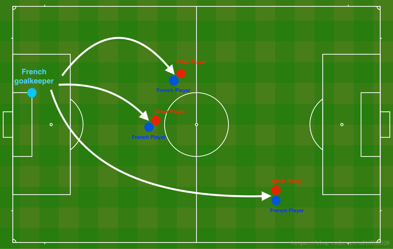
Problem Statement: You have just been hired as an AI expert by the French Football Corporation. They would like you to recommend positions where France's goal keeper should kick the ball so that the French team's players can then hit it with their head.

The goal keeper kicks the ball in the air, the players of each team are fighting to hit the ball with their head
They give you the following 2D dataset from France's past 10 games.
train_X, train_Y, test_X, test_Y = load_2D_dataset()

Each dot corresponds to a position on the football field where a football player has hit the ball with his/her head after the French goal keeper has shot the ball from the left side of the football field.
- If the dot is blue, it means the French player managed to hit the ball with his/her head
- If the dot is red, it means the other team's player hit the ball with their head
Your goal: Use a deep learning model to find the positions on the field where the goalkeeper should kick the ball.
Analysis of the dataset: This dataset is a little noisy, but it looks like a diagonal line separating the upper left half (blue) from the lower right half (red) would work well.
You will first try a non-regularized model. Then you'll learn how to regularize it and decide which model you will choose to solve the French Football Corporation's problem.
1 - Non-regularized model
You will use the following neural network (already implemented for you below). This model can be used:
- in regularization mode -- by setting the
lambdinput to a non-zero value. We use "lambd" instead of "lambda" because "lambda" is a reserved keyword in Python. - in dropout mode -- by setting the
keep_probto a value less than one
You will first try the model without any regularization. Then, you will implement:
- L2 regularization -- functions: "
compute_cost_with_regularization()" and "backward_propagation_with_regularization()" - Dropout -- functions: "
forward_propagation_with_dropout()" and "backward_propagation_with_dropout()"
In each part, you will run this model with the correct inputs so that it calls the functions you've implemented. Take a look at the code below to familiarize yourself with the model.
def model(X, Y, learning_rate = 0.3, num_iterations = 30000, print_cost = True, lambd = 0, keep_prob = 1):
"""
Implements a three-layer neural network: LINEAR->RELU->LINEAR->RELU->LINEAR->SIGMOID.
Arguments:
X -- input data, of shape (input size, number of examples)
Y -- true "label" vector (1 for blue dot / 0 for red dot), of shape (output size, number of examples)
learning_rate -- learning rate of the optimization
num_iterations -- number of iterations of the optimization loop
print_cost -- If True, print the cost every 10000 iterations
lambd -- regularization hyperparameter, scalar
keep_prob - probability of keeping a neuron active during drop-out, scalar.
Returns:
parameters -- parameters learned by the model. They can then be used to predict.
"""
grads = {}
costs = [] # to keep track of the cost
m = X.shape[1] # number of examples
layers_dims = [X.shape[0], 20, 3, 1]
# Initialize parameters dictionary.
parameters = initialize_parameters(layers_dims)
# Loop (gradient descent)
for i in range(0, num_iterations):
# Forward propagation: LINEAR -> RELU -> LINEAR -> RELU -> LINEAR -> SIGMOID.
if keep_prob == 1:
a3, cache = forward_propagation(X, parameters)
elif keep_prob < 1:
a3, cache = forward_propagation_with_dropout(X, parameters, keep_prob)
# Cost function
if lambd == 0:
cost = compute_cost(a3, Y)
else:
cost = compute_cost_with_regularization(a3, Y, parameters, lambd)
# Backward propagation.
assert(lambd==0 or keep_prob==1) # it is possible to use both L2 regularization and dropout,
# but this assignment will only explore one at a time
if lambd == 0 and keep_prob == 1:
grads = backward_propagation(X, Y, cache)
elif lambd != 0:
grads = backward_propagation_with_regularization(X, Y, cache, lambd)
elif keep_prob < 1:
grads = backward_propagation_with_dropout(X, Y, cache, keep_prob)
# Update parameters.
parameters = update_parameters(parameters, grads, learning_rate)
# Print the loss every 10000 iterations
if print_cost and i % 10000 == 0:
print("Cost after iteration {}: {}".format(i, cost))
if print_cost and i % 1000 == 0:
costs.append(cost)
# plot the cost
plt.plot(costs)
plt.ylabel('cost')
plt.xlabel('iterations (x1,000)')
plt.title("Learning rate =" + str(learning_rate))
plt.show()
return parameters
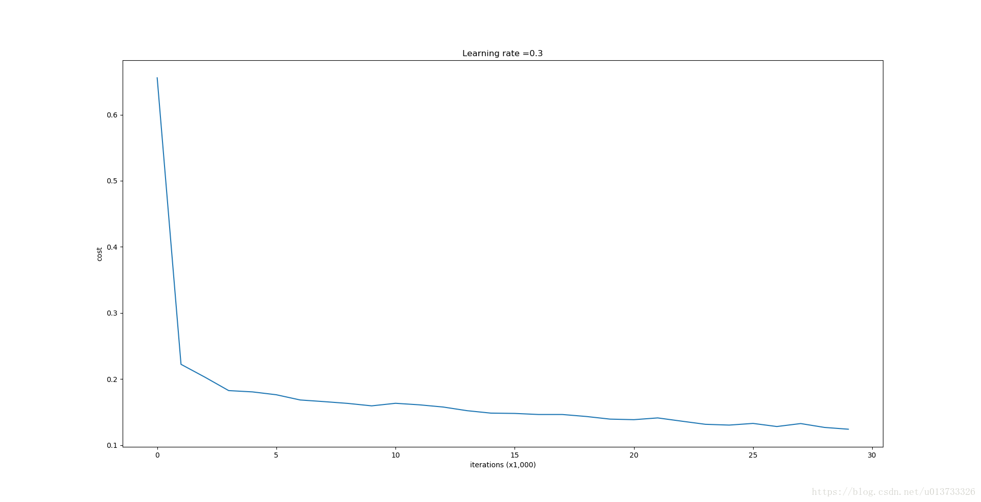
Let's train the model without any regularization, and observe the accuracy on the train/test sets.
parameters = model(train_X, train_Y)
print ("On the training set:")
predictions_train = predict(train_X, train_Y, parameters)
print ("On the test set:")
predictions_test = predict(test_X, test_Y, parameters)

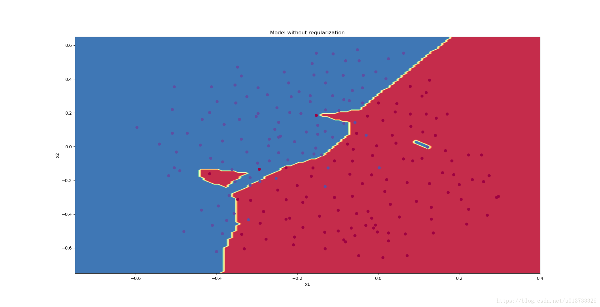
The train accuracy is 94.8% while the test accuracy is 91.5%. This is the baseline model (you will observe the impact of regularization on this model). Run the following code to plot the decision boundary of your model.
plt.title("Model without regularization")
axes = plt.gca()
axes.set_xlim([-0.75,0.40])
axes.set_ylim([-0.75,0.65])
plot_decision_boundary(lambda x: predict_dec(parameters, x.T), train_X, train_Y)

The non-regularized model is obviously overfitting the training set. It is fitting the noisy points! Lets now look at two techniques to reduce overfitting.
2 - L2 Regularization
The standard way to avoid overfitting is called L2 regularization. It consists of appropriately modifying your cost function, from:
Let's modify your cost and observe the consequences.
Exercise: Implement compute_cost_with_regularization() which computes the cost given by formula (2). To calculate ∑k∑jW[l]2k,j∑k∑jWk,j[l]2 , use :
np.sum(np.square(Wl)) Note that you have to do this for W[1]W[1], W[2]W[2] and W[3]W[3], then sum the three terms and multiply by 1mλ21mλ2.
# GRADED FUNCTION: compute_cost_with_regularization
def compute_cost_with_regularization(A3, Y, parameters, lambd):
"""
Implement the cost function with L2 regularization. See formula (2) above.
Arguments:
A3 -- post-activation, output of forward propagation, of shape (output size, number of examples)
Y -- "true" labels vector, of shape (output size, number of examples)
parameters -- python dictionary containing parameters of the model
Returns:
cost - value of the regularized loss function (formula (2))
"""
m = Y.shape[1]
W1 = parameters["W1"]
W2 = parameters["W2"]
W3 = parameters["W3"]
cross_entropy_cost = compute_cost(A3, Y) # This gives you the cross-entropy part of the cost
### START CODE HERE ### (approx. 1 line)
L2_regularization_cost = lambd * (np.sum(np.square(W1)) + np.sum(np.square(W2)) + np.sum(np.square(W3))) / (2 * m)
### END CODER HERE ###
cost = cross_entropy_cost + L2_regularization_cost
return cost
A3, Y_assess, parameters = compute_cost_with_regularization_test_case()
print("cost = " + str(compute_cost_with_regularization(A3, Y_assess, parameters, lambd = 0.1)))
Expected Output:
| cost | 1.78648594516 |
Of course, because you changed the cost, you have to change backward propagation as well! All the gradients have to be computed with respect to this new cost.
Exercise: Implement the changes needed in backward propagation to take into account regularization. The changes only concern dW1, dW2 and dW3. For each, you have to add the regularization term's gradient (ddW(12λmW2)=λmWddW(12λmW2)=λmW).
# GRADED FUNCTION: backward_propagation_with_regularization
def backward_propagation_with_regularization(X, Y, cache, lambd):
"""
Implements the backward propagation of our baseline model to which we added an L2 regularization.
Arguments:
X -- input dataset, of shape (input size, number of examples)
Y -- "true" labels vector, of shape (output size, number of examples)
cache -- cache output from forward_propagation()
lambd -- regularization hyperparameter, scalar
Returns:
gradients -- A dictionary with the gradients with respect to each parameter, activation and pre-activation variables
"""
m = X.shape[1]
(Z1, A1, W1, b1, Z2, A2, W2, b2, Z3, A3, W3, b3) = cache
dZ3 = A3 - Y
### START CODE HERE ### (approx. 1 line)
dW3 = 1./m * np.dot(dZ3, A2.T) +(lambd*W3)/m
### END CODE HERE ###
db3 = 1./m * np.sum(dZ3, axis=1, keepdims = True)
dA2 = np.dot(W3.T, dZ3)
dZ2 = np.multiply(dA2, np.int64(A2 > 0))
### START CODE HERE ### (approx. 1 line)
dW2 = 1./m * np.dot(dZ2, A1.T) + (lambd*W2)/m
### END CODE HERE ###
db2 = 1./m * np.sum(dZ2, axis=1, keepdims = True)
dA1 = np.dot(W2.T, dZ2)
dZ1 = np.multiply(dA1, np.int64(A1 > 0))
### START CODE HERE ### (approx. 1 line)
dW1 = 1./m * np.dot(dZ1, X.T) + (lambd*W1)/m
### END CODE HERE ###
db1 = 1./m * np.sum(dZ1, axis=1, keepdims = True)
gradients = {"dZ3": dZ3, "dW3": dW3, "db3": db3,"dA2": dA2,
"dZ2": dZ2, "dW2": dW2, "db2": db2, "dA1": dA1,
"dZ1": dZ1, "dW1": dW1, "db1": db1}
return gradients
X_assess, Y_assess, cache = backward_propagation_with_regularization_test_case()
grads = backward_propagation_with_regularization(X_assess, Y_assess, cache, lambd = 0.7)
print ("dW1 = "+ str(grads["dW1"]))
print ("dW2 = "+ str(grads["dW2"]))
print ("dW3 = "+ str(grads["dW3"]))
Expected Output:
| dW1 | [[-0.25604646 0.12298827 -0.28297129] [-0.17706303 0.34536094 -0.4410571 ]] |
| dW2 | [[ 0.79276486 0.85133918] [-0.0957219 -0.01720463] [-0.13100772 -0.03750433]] |
| dW3 | [[-1.77691347 -0.11832879 -0.09397446]] |
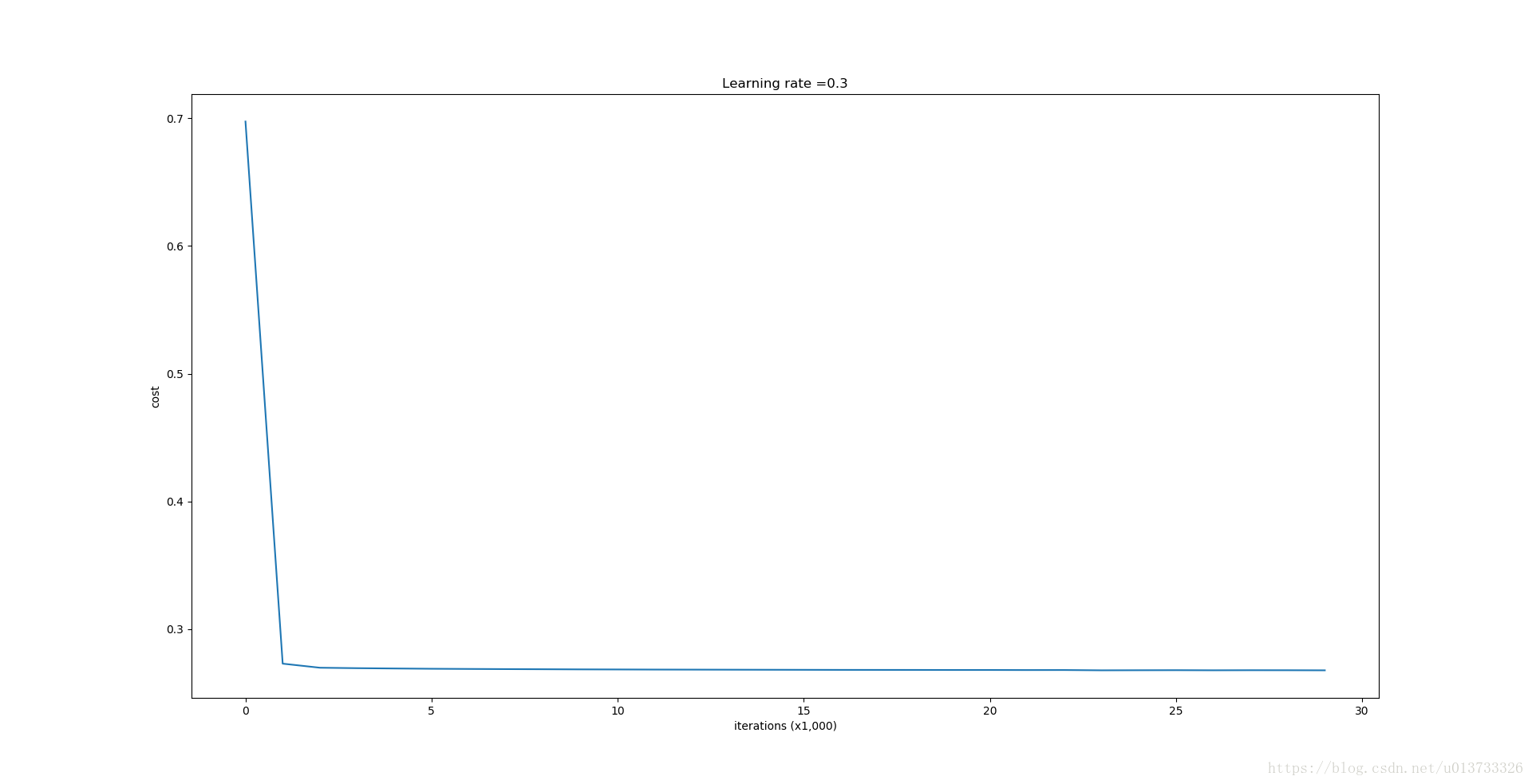
Let's now run the model with L2 regularization (λ=0.7)(λ=0.7). The model() function will call:
compute_cost_with_regularizationinstead ofcompute_costbackward_propagation_with_regularizationinstead ofbackward_propagation
parameters = model(train_X, train_Y, lambd = 0.7)
print ("On the train set:")
predictions_train = predict(train_X, train_Y, parameters)
print ("On the test set:")
predictions_test = predict(test_X, test_Y, parameters)

Congrats, the test set accuracy increased to 93%. You have saved the French football team!
You are not overfitting the training data anymore. Let's plot the decision boundary.
plt.title("Model with L2-regularization")
axes = plt.gca()
axes.set_xlim([-0.75,0.40])
axes.set_ylim([-0.75,0.65])
plot_decision_boundary(lambda x: predict_dec(parameters, x.T), train_X, train_Y)

Observations:
- The value of λλ is a hyperparameter that you can tune using a dev set.
- L2 regularization makes your decision boundary smoother. If λλ is too large, it is also possible to "oversmooth", resulting in a model with high bias.
What is L2-regularization actually doing?:
L2-regularization relies on the assumption that a model with small weights is simpler than a model with large weights. Thus, by penalizing the square values of the weights in the cost function you drive all the weights to smaller values. It becomes too costly for the cost to have large weights! This leads to a smoother model in which the output changes more slowly as the input changes.
What you should remember -- the implications of L2-regularization on:
- The cost computation:
- A regularization term is added to the cost
- The backpropagation function:
- There are extra terms in the gradients with respect to weight matrices
- Weights end up smaller ("weight decay"):
- Weights are pushed to smaller values.
3 - Dropout
Finally, dropout is a widely used regularization technique that is specific to deep learning. It randomly shuts down some neurons in each iteration. Watch these two videos to see what this means!
At each iteration, you shut down (= set to zero) each neuron of a layer with probability 1−keep_prob1−keep_prob or keep it with probability keep_probkeep_prob (50% here). The dropped neurons don't contribute to the training in both the forward and backward propagations of the iteration.
1st1st layer: we shut down on average 40% of the neurons. 3rd3rd layer: we shut down on average 20% of the neurons.
When you shut some neurons down, you actually modify your model. The idea behind drop-out is that at each iteration, you train a different model that uses only a subset of your neurons. With dropout, your neurons thus become less sensitive to the activation of one other specific neuron, because that other neuron might be shut down at any time.
3.1 - Forward propagation with dropout
Exercise: Implement the forward propagation with dropout. You are using a 3 layer neural network, and will add dropout to the first and second hidden layers. We will not apply dropout to the input layer or output layer.
Instructions: You would like to shut down some neurons in the first and second layers. To do that, you are going to carry out 4 Steps:
- In lecture, we dicussed creating a variable d[1]d[1] with the same shape as a[1]a[1] using
np.random.rand()to randomly get numbers between 0 and 1. Here, you will use a vectorized implementation, so create a random matrix D[1]=[d[1](1)d[1](2)...d[1](m)]D[1]=[d[1](1)d[1](2)...d[1](m)] of the same dimension as A[1]A[1]. - Set each entry of D[1]D[1] to be 0 with probability (
1-keep_prob) or 1 with probability (keep_prob), by thresholding values in D[1]D[1] appropriately. Hint: to set all the entries of a matrix X to 0 (if entry is less than 0.5) or 1 (if entry is more than 0.5) you would do:X = (X < 0.5). Note that 0 and 1 are respectively equivalent to False and True. - Set A[1]A[1] to A[1]∗D[1]A[1]∗D[1]. (You are shutting down some neurons). You can think of D[1]D[1] as a mask, so that when it is multiplied with another matrix, it shuts down some of the values.
- Divide A[1]A[1] by
keep_prob. By doing this you are assuring that the result of the cost will still have the same expected value as without drop-out. (This technique is also called inverted dropout.)
# GRADED FUNCTION: forward_propagation_with_dropout
def forward_propagation_with_dropout(X, parameters, keep_prob = 0.5):
"""
Implements the forward propagation: LINEAR -> RELU + DROPOUT -> LINEAR -> RELU + DROPOUT -> LINEAR -> SIGMOID.
Arguments:
X -- input dataset, of shape (2, number of examples)
parameters -- python dictionary containing your parameters "W1", "b1", "W2", "b2", "W3", "b3":
W1 -- weight matrix of shape (20, 2)
b1 -- bias vector of shape (20, 1)
W2 -- weight matrix of shape (3, 20)
b2 -- bias vector of shape (3, 1)
W3 -- weight matrix of shape (1, 3)
b3 -- bias vector of shape (1, 1)
keep_prob - probability of keeping a neuron active during drop-out, scalar
Returns:
A3 -- last activation value, output of the forward propagation, of shape (1,1)
cache -- tuple, information stored for computing the backward propagation
"""
np.random.seed(1)
# retrieve parameters
W1 = parameters["W1"]
b1 = parameters["b1"]
W2 = parameters["W2"]
b2 = parameters["b2"]
W3 = parameters["W3"]
b3 = parameters["b3"]
# LINEAR -> RELU -> LINEAR -> RELU -> LINEAR -> SIGMOID
Z1 = np.dot(W1, X) + b1
A1 = relu(Z1)
### START CODE HERE ### (approx. 4 lines) # Steps 1-4 below correspond to the Steps 1-4 described above.
D1 = np.random.randn(A1.shape[0],A1.shape[1]) # Step 1: initialize matrix D1 = np.random.rand(..., ...)
D1 = np.round(D1) # Step 2: convert entries of D1 to 0 or 1 (using keep_prob as the threshold)
A1 = A1*D1 # Step 3: shut down some neurons of A1
A1 =A1/keep_prob # Step 4: scale the value of neurons that haven't been shut down
### END CODE HERE ###
Z2 = np.dot(W2, A1) + b2
A2 = relu(Z2)
### START CODE HERE ### (approx. 4 lines)
D2 = np.random.randn(A2.shape[0],A2.shape[1]) # Step 1: initialize matrix D2 = np.random.rand(..., ...)
D2 = np.round(D2) # Step 2: convert entries of D2 to 0 or 1 (using keep_prob as the threshold)
A2 = A2*D2 # Step 3: shut down some neurons of A2
A2 = A2/keep_prob # Step 4: scale the value of neurons that haven't been shut down
### END CODE HERE ###
Z3 = np.dot(W3, A2) + b3
A3 = sigmoid(Z3)
cache = (Z1, D1, A1, W1, b1, Z2, D2, A2, W2, b2, Z3, A3, W3, b3)
return A3, cache
X_assess, parameters = forward_propagation_with_dropout_test_case()
A3, cache = forward_propagation_with_dropout(X_assess, parameters, keep_prob = 0.7)
print ("A3 = " + str(A3))
Expected Output:
| A3 | [[ 0.36974721 0.00305176 0.04565099 0.49683389 0.36974721]] |
3.2 - Backward propagation with dropout
Exercise: Implement the backward propagation with dropout. As before, you are training a 3 layer network. Add dropout to the first and second hidden layers, using the masks D[1]D[1] and D[2]D[2] stored in the cache.
Instruction: Backpropagation with dropout is actually quite easy. You will have to carry out 2 Steps:
- You had previously shut down some neurons during forward propagation, by applying a mask D[1]D[1] to
A1. In backpropagation, you will have to shut down the same neurons, by reapplying the same mask D[1]D[1] todA1. - During forward propagation, you had divided
A1bykeep_prob. In backpropagation, you'll therefore have to dividedA1bykeep_probagain (the calculus interpretation is that if A[1]A[1] is scaled bykeep_prob, then its derivative dA[1]dA[1] is also scaled by the samekeep_prob).
# GRADED FUNCTION: backward_propagation_with_dropout
def backward_propagation_with_dropout(X, Y, cache, keep_prob):
"""
Implements the backward propagation of our baseline model to which we added dropout.
Arguments:
X -- input dataset, of shape (2, number of examples)
Y -- "true" labels vector, of shape (output size, number of examples)
cache -- cache output from forward_propagation_with_dropout()
keep_prob - probability of keeping a neuron active during drop-out, scalar
Returns:
gradients -- A dictionary with the gradients with respect to each parameter, activation and pre-activation variables
"""
m = X.shape[1]
(Z1, D1, A1, W1, b1, Z2, D2, A2, W2, b2, Z3, A3, W3, b3) = cache
dZ3 = A3 - Y
dW3 = 1./m * np.dot(dZ3, A2.T)
db3 = 1./m * np.sum(dZ3, axis=1, keepdims = True)
dA2 = np.dot(W3.T, dZ3)
### START CODE HERE ### (≈ 2 lines of code)
dA2 =dA2*D2 # Step 1: Apply mask D2 to shut down the same neurons as during the forward propagation
dA2 = dA2/keep_prob # Step 2: Scale the value of neurons that haven't been shut down
### END CODE HERE ###
dZ2 = np.multiply(dA2, np.int64(A2 > 0))
dW2 = 1./m * np.dot(dZ2, A1.T)
db2 = 1./m * np.sum(dZ2, axis=1, keepdims = True)
dA1 = np.dot(W2.T, dZ2)
### START CODE HERE ### (≈ 2 lines of code)
dA1 = dA1*D1 # Step 1: Apply mask D1 to shut down the same neurons as during the forward propagation
dA1 = dA1/keep_prob # Step 2: Scale the value of neurons that haven't been shut down
### END CODE HERE ###
dZ1 = np.multiply(dA1, np.int64(A1 > 0))
dW1 = 1./m * np.dot(dZ1, X.T)
db1 = 1./m * np.sum(dZ1, axis=1, keepdims = True)
gradients = {"dZ3": dZ3, "dW3": dW3, "db3": db3,"dA2": dA2,
"dZ2": dZ2, "dW2": dW2, "db2": db2, "dA1": dA1,
"dZ1": dZ1, "dW1": dW1, "db1": db1}
return gradients
X_assess, Y_assess, cache = backward_propagation_with_dropout_test_case()
gradients = backward_propagation_with_dropout(X_assess, Y_assess, cache, keep_prob = 0.8)
print ("dA1 = " + str(gradients["dA1"]))
print ("dA2 = " + str(gradients["dA2"]))
Expected Output:
| dA1 | [[ 0.36544439 0. -0.00188233 0. -0.17408748] [ 0.65515713 0. -0.00337459 0. -0. ]] |
| dA2 | [[ 0.58180856 0. -0.00299679 0. -0.27715731] [ 0. 0.53159854 -0. 0.53159854 -0.34089673] [ 0. 0. -0.00292733 0. -0. ]] |
Let's now run the model with dropout (keep_prob = 0.86). It means at every iteration you shut down each neurons of layer 1 and 2 with 14% probability. The function model() will now call:
forward_propagation_with_dropoutinstead offorward_propagation.backward_propagation_with_dropoutinstead ofbackward_propagation.
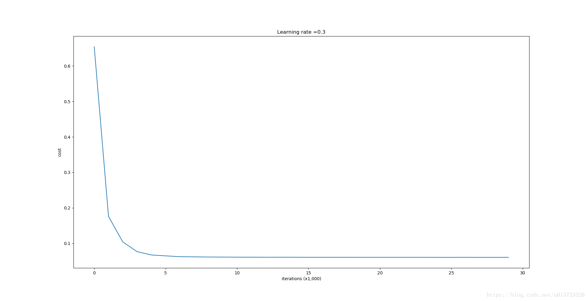
parameters = model(train_X, train_Y, keep_prob = 0.86, learning_rate = 0.3)
print ("On the train set:")
predictions_train = predict(train_X, train_Y, parameters)
print ("On the test set:")
predictions_test = predict(test_X, test_Y, parameters)

Dropout works great! The test accuracy has increased again (to 95%)! Your model is not overfitting the training set and does a great job on the test set. The French football team will be forever grateful to you!
Run the code below to plot the decision boundary.
plt.title("Model with dropout")
axes = plt.gca()
axes.set_xlim([-0.75,0.40])
axes.set_ylim([-0.75,0.65])
plot_decision_boundary(lambda x: predict_dec(parameters, x.T), train_X, train_Y)

Note:
- A common mistake when using dropout is to use it both in training and testing. You should use dropout (randomly eliminate nodes) only in training.
- Deep learning frameworks like tensorflow, PaddlePaddle, keras or caffe come with a dropout layer implementation. Don't stress - you will soon learn some of these frameworks.
What you should remember about dropout:
- Dropout is a regularization technique.
- You only use dropout during training. Don't use dropout (randomly eliminate nodes) during test time.
- Apply dropout both during forward and backward propagation.
- During training time, divide each dropout layer by keep_prob to keep the same expected value for the activations. For example, if keep_prob is 0.5, then we will on average shut down half the nodes, so the output will be scaled by 0.5 since only the remaining half are contributing to the solution. Dividing by 0.5 is equivalent to multiplying by 2. Hence, the output now has the same expected value. You can check that this works even when keep_prob is other values than 0.5.
4 - Conclusions
Here are the results of our three models:
| model | train accuracy | test accuracy |
| 3-layer NN without regularization | 95% | 91.5% |
| 3-layer NN with L2-regularization | 94% | 93% |
| 3-layer NN with dropout | 93% | 95% |
Note that regularization hurts training set performance! This is because it limits the ability of the network to overfit to the training set. But since it ultimately gives better test accuracy, it is helping your system.
Congratulations for finishing this assignment! And also for revolutionizing French football. :-)
What we want you to remember from this notebook:
- Regularization will help you reduce overfitting.
- Regularization will drive your weights to lower values.
- L2 regularization and Dropout are two very effective regularization techniques.
别人的中文版----------------------------------------------------------------------------------------------------------------------------------------------------------------------------------------------------
正则化模型
Problem Statement: You have just been hired as an AI expert by the French Football Corporation. They would like you to recommend positions where France’s goal keeper should kick the ball so that the French team’s players can then hit it with their head.
问题描述:假设你现在是一个AI专家,你需要设计一个模型,可以用于推荐在足球场中守门员将球发至哪个位置可以让本队的球员抢到球的可能性更大。说白了,实际上就是一个二分类,一半是己方抢到球,一半就是对方抢到球,我们来看一下这个图:
读取并绘制数据集
我们来加载并查看一下我们的数据集:
train_X, train_Y, test_X, test_Y = reg_utils.load_2D_dataset(is_plot=True)- 1
执行结果:
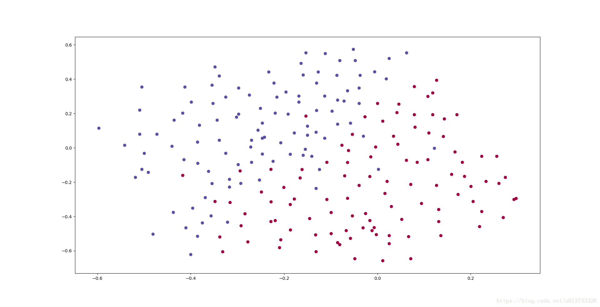
每一个点代表球落下的可能的位置,蓝色代表己方的球员会抢到球,红色代表对手的球员会抢到球,我们要做的就是使用模型来画出一条线,来找到适合我方球员能抢到球的位置。
我们要做以下三件事,来对比出不同的模型的优劣:
- 不使用正则化
- 使用正则化
2.1 使用L2正则化
2.2 使用随机节点删除
我们来看一下我们的模型:
- 正则化模式 - 将lambd输入设置为非零值。 我们使用“lambd”而不是“lambda”,因为“lambda”是Python中的保留关键字。
- 随机删除节点 - 将keep_prob设置为小于1的值
def model(X,Y,learning_rate=0.3,num_iterations=30000,print_cost=True,is_plot=True,lambd=0,keep_prob=1): """ 实现一个三层的神经网络:LINEAR ->RELU -> LINEAR -> RELU -> LINEAR -> SIGMOID 参数: X - 输入的数据,维度为(2, 要训练/测试的数量) Y - 标签,【0(蓝色) | 1(红色)】,维度为(1,对应的是输入的数据的标签) learning_rate - 学习速率 num_iterations - 迭代的次数 print_cost - 是否打印成本值,每迭代10000次打印一次,但是每1000次记录一个成本值 is_polt - 是否绘制梯度下降的曲线图 lambd - 正则化的超参数,实数 keep_prob - 随机删除节点的概率 返回 parameters - 学习后的参数 """ grads = {} costs = [] m = X.shape[1] layers_dims = [X.shape[0],20,3,1] #初始化参数 parameters = reg_utils.initialize_parameters(layers_dims) #开始学习 for i in range(0,num_iterations): #前向传播 ##是否随机删除节点 if keep_prob == 1: ###不随机删除节点 a3 , cache = reg_utils.forward_propagation(X,parameters) elif keep_prob < 1: ###随机删除节点 a3 , cache = forward_propagation_with_dropout(X,parameters,keep_prob) else: print("keep_prob参数错误!程序退出。") exit #计算成本 ## 是否使用二范数 if lambd == 0: ###不使用L2正则化 cost = reg_utils.compute_cost(a3,Y) else: ###使用L2正则化 cost = compute_cost_with_regularization(a3,Y,parameters,lambd) #反向传播 ##可以同时使用L2正则化和随机删除节点,但是本次实验不同时使用。 assert(lambd == 0 or keep_prob ==1) ##两个参数的使用情况 if (lambd == 0 and keep_prob == 1): ### 不使用L2正则化和不使用随机删除节点 grads = reg_utils.backward_propagation(X,Y,cache) elif lambd != 0: ### 使用L2正则化,不使用随机删除节点 grads = backward_propagation_with_regularization(X, Y, cache, lambd) elif keep_prob < 1: ### 使用随机删除节点,不使用L2正则化 grads = backward_propagation_with_dropout(X, Y, cache, keep_prob) #更新参数 parameters = reg_utils.update_parameters(parameters, grads, learning_rate) #记录并打印成本 if i % 1000 == 0: ## 记录成本 costs.append(cost) if (print_cost and i % 10000 == 0): #打印成本 print("第" + str(i) + "次迭代,成本值为:" + str(cost)) #是否绘制成本曲线图 if is_plot: plt.plot(costs) plt.ylabel('cost') plt.xlabel('iterations (x1,000)') plt.title("Learning rate =" + str(learning_rate)) plt.show() #返回学习后的参数 return parameters- 1
- 2
- 3
- 4
- 5
- 6
- 7
- 8
- 9
- 10
- 11
- 12
- 13
- 14
- 15
- 16
- 17
- 18
- 19
- 20
- 21
- 22
- 23
- 24
- 25
- 26
- 27
- 28
- 29
- 30
- 31
- 32
- 33
- 34
- 35
- 36
- 37
- 38
- 39
- 40
- 41
- 42
- 43
- 44
- 45
- 46
- 47
- 48
- 49
- 50
- 51
- 52
- 53
- 54
- 55
- 56
- 57
- 58
- 59
- 60
- 61
- 62
- 63
- 64
- 65
- 66
- 67
- 68
- 69
- 70
- 71
- 72
- 73
- 74
- 75
- 76
- 77
- 78
- 79
- 80
- 81
- 82
- 83
我们来先看一下不使用正则化下模型的效果:
不使用正则化
parameters = model(train_X, train_Y,is_plot=True)
print("训练集:")
predictions_train = reg_utils.predict(train_X, train_Y, parameters)
print("测试集:")
predictions_test = reg_utils.predict(test_X, test_Y, parameters)- 1
- 2
- 3
- 4
- 5
执行结果:
第0次迭代,成本值为:0.655741252348
第10000次迭代,成本值为:0.163299875257
第20000次迭代,成本值为:0.138516424233 训练集: Accuracy: 0.947867298578 测试集: Accuracy: 0.915- 1
- 2
- 3
- 4
- 5
- 6
- 7
我们可以看到,对于训练集,精确度为94%;而对于测试集,精确度为91.5%。接下来,我们将分割曲线画出来:
plt.title("Model without regularization")
axes = plt.gca()
axes.set_xlim([-0.75,0.40])
axes.set_ylim([-0.75,0.65]) reg_utils.plot_decision_boundary(lambda x: reg_utils.predict_dec(parameters, x.T), train_X, train_Y)- 1
- 2
- 3
- 4
- 5
执行结果:
从图中可以看出,在无正则化时,分割曲线有了明显的过拟合特性。接下来,我们使用L2正则化:
使用正则化
L2正则化
避免过度拟合的标准方法称为L2正则化,它包括适当修改你的成本函数,我们从原来的成本函数(1)到现在的函数(2):
计算∑k∑jW[l]2k,j∑k∑jWk,j[l]2的代码为:
np.sum(np.square(Wl))- 1
需要注意的是在前向传播中我们对 W[1]W[1], W[2]W[2] 和W[3]W[3]这三个项进行操作,将这三个项相加并乘以 1mλ21mλ2。在后向传播中,使用ddW(12λmW2)=λmWddW(12λmW2)=λmW计算梯度。
我们下面就开始写相关的函数:
def compute_cost_with_regularization(A3,Y,parameters,lambd):
    """ 实现公式2的L2正则化计算成本 参数: A3 - 正向传播的输出结果,维度为(输出节点数量,训练/测试的数量) Y - 标签向量,与数据一一对应,维度为(输出节点数量,训练/测试的数量) parameters - 包含模型学习后的参数的字典 返回: cost - 使用公式2计算出来的正则化损失的值 """ m = Y.shape[1] W1 = parameters["W1"] W2 = parameters["W2"] W3 = parameters["W3"] cross_entropy_cost = reg_utils.compute_cost(A3,Y) L2_regularization_cost = lambd * (np.sum(np.square(W1)) + np.sum(np.square(W2)) + np.sum(np.square(W3))) / (2 * m) cost = cross_entropy_cost + L2_regularization_cost return cost #当然,因为改变了成本函数,我们也必须改变向后传播的函数, 所有的梯度都必须根据这个新的成本值来计算。 def backward_propagation_with_regularization(X, Y, cache, lambd): """ 实现我们添加了L2正则化的模型的后向传播。 参数: X - 输入数据集,维度为(输入节点数量,数据集里面的数量) Y - 标签,维度为(输出节点数量,数据集里面的数量) cache - 来自forward_propagation()的cache输出 lambda - regularization超参数,实数 返回: gradients - 一个包含了每个参数、激活值和预激活值变量的梯度的字典 """ m = X.shape[1] (Z1, A1, W1, b1, Z2, A2, W2, b2, Z3, A3, W3, b3) = cache dZ3 = A3 - Y dW3 = (1 / m) * np.dot(dZ3,A2.T) + ((lambd * W3) / m ) db3 = (1 / m) * np.sum(dZ3,axis=1,keepdims=True) dA2 = np.dot(W3.T,dZ3) dZ2 = np.multiply(dA2,np.int64(A2 > 0)) dW2 = (1 / m) * np.dot(dZ2,A1.T) + ((lambd * W2) / m) db2 = (1 / m) * np.sum(dZ2,axis=1,keepdims=True) dA1 = np.dot(W2.T,dZ2) dZ1 = np.multiply(dA1,np.int64(A1 > 0)) dW1 = (1 / m) * np.dot(dZ1,X.T) + ((lambd * W1) / m) db1 = (1 / m) * np.sum(dZ1,axis=1,keepdims=True) gradients = {"dZ3": dZ3, "dW3": dW3, "db3": db3, "dA2": dA2, "dZ2": dZ2, "dW2": dW2, "db2": db2, "dA1": dA1, "dZ1": dZ1, "dW1": dW1, "db1": db1} return gradients
我们来直接放到模型中跑一下:
parameters = model(train_X, train_Y, lambd=0.7,is_plot=True)
print("使用正则化,训练集:") predictions_train = reg_utils.predict(train_X, train_Y, parameters) print("使用正则化,测试集:") predictions_test = reg_utils.predict(test_X, test_Y, parameters)执行结果:
第0次迭代,成本值为:0.697448449313
第10000次迭代,成本值为:0.268491887328
第20000次迭代,成本值为:0.268091633713 使用正则化,训练集: Accuracy: 0.938388625592 使用正则化,测试集: Accuracy: 0.93- 1
- 2
- 3
- 4
- 5
- 6
- 7
我们来看一下分类的结果吧~
plt.title("Model with L2-regularization")
axes = plt.gca()
axes.set_xlim([-0.75,0.40])
axes.set_ylim([-0.75,0.65]) reg_utils.plot_decision_boundary(lambda x: reg_utils.predict_dec(parameters, x.T), train_X, train_Y)- 1
- 2
- 3
- 4
- 5
执行结果:
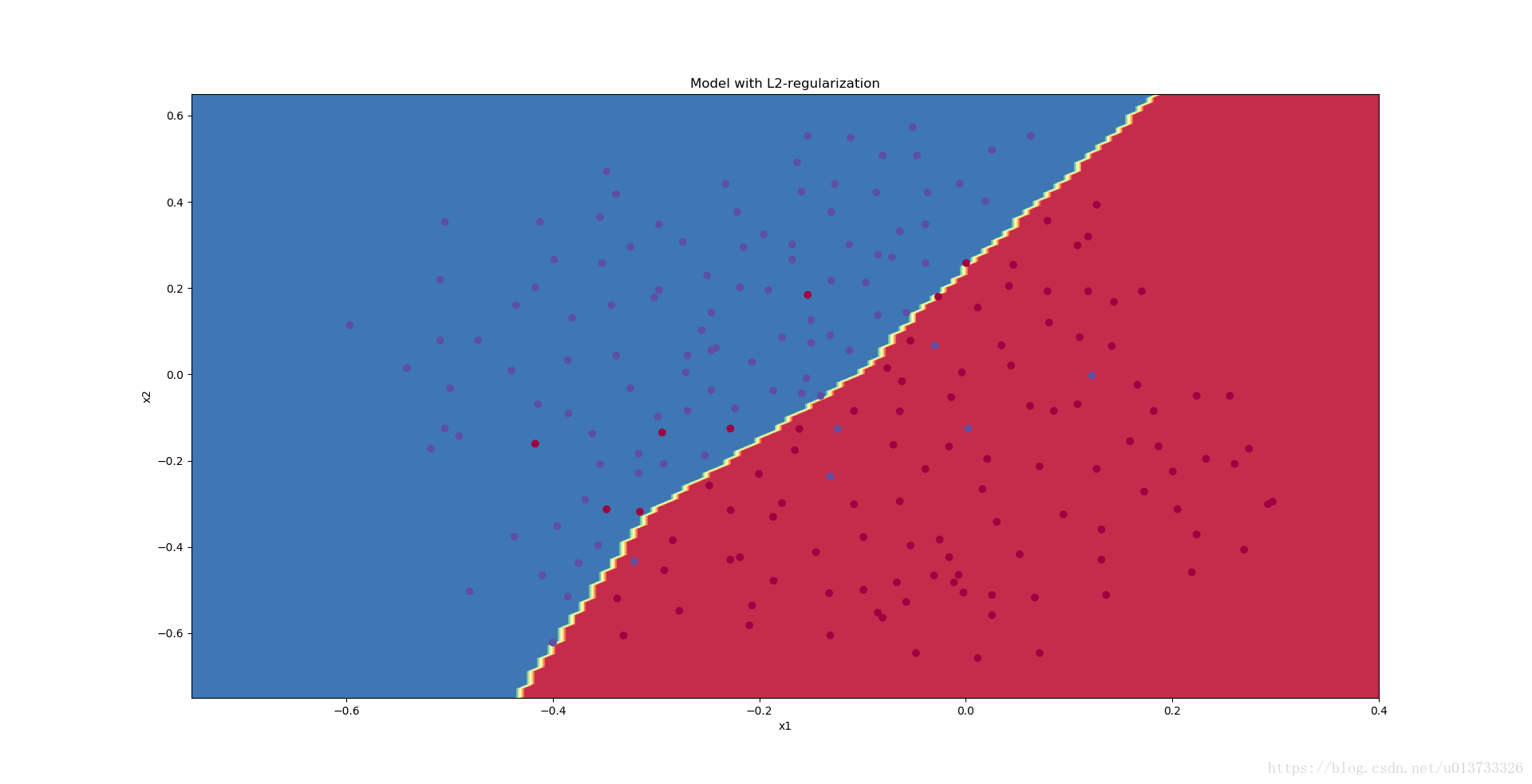
λ的值是可以使用开发集调整时的超参数。L2正则化会使决策边界更加平滑。如果λ太大,也可能会“过度平滑”,从而导致模型高偏差。L2正则化实际上在做什么?L2正则化依赖于较小权重的模型比具有较大权重的模型更简单这样的假设,因此,通过削减成本函数中权重的平方值,可以将所有权重值逐渐改变到到较小的值。权值数值高的话会有更平滑的模型,其中输入变化时输出变化更慢,但是你需要花费更多的时间。L2正则化对以下内容有影响:
- 成本计算 : 正则化的计算需要添加到成本函数中
- 反向传播功能 :在权重矩阵方面,梯度计算时也要依据正则化来做出相应的计算
- 重量变小(“重量衰减”) :权重被逐渐改变到较小的值。
随机删除节点
最后,我们使用Dropout来进行正则化,Dropout的原理就是每次迭代过程中随机将其中的一些节点失效。当我们关闭一些节点时,我们实际上修改了我们的模型。背后的想法是,在每次迭代时,我们都会训练一个只使用一部分神经元的不同模型。随着迭代次数的增加,我们的模型的节点会对其他特定节点的激活变得不那么敏感,因为其他节点可能在任何时候会失效。我们来看看下面两个GIF图,图有点大,加载不出来请【点我下载(11.3MB)】:
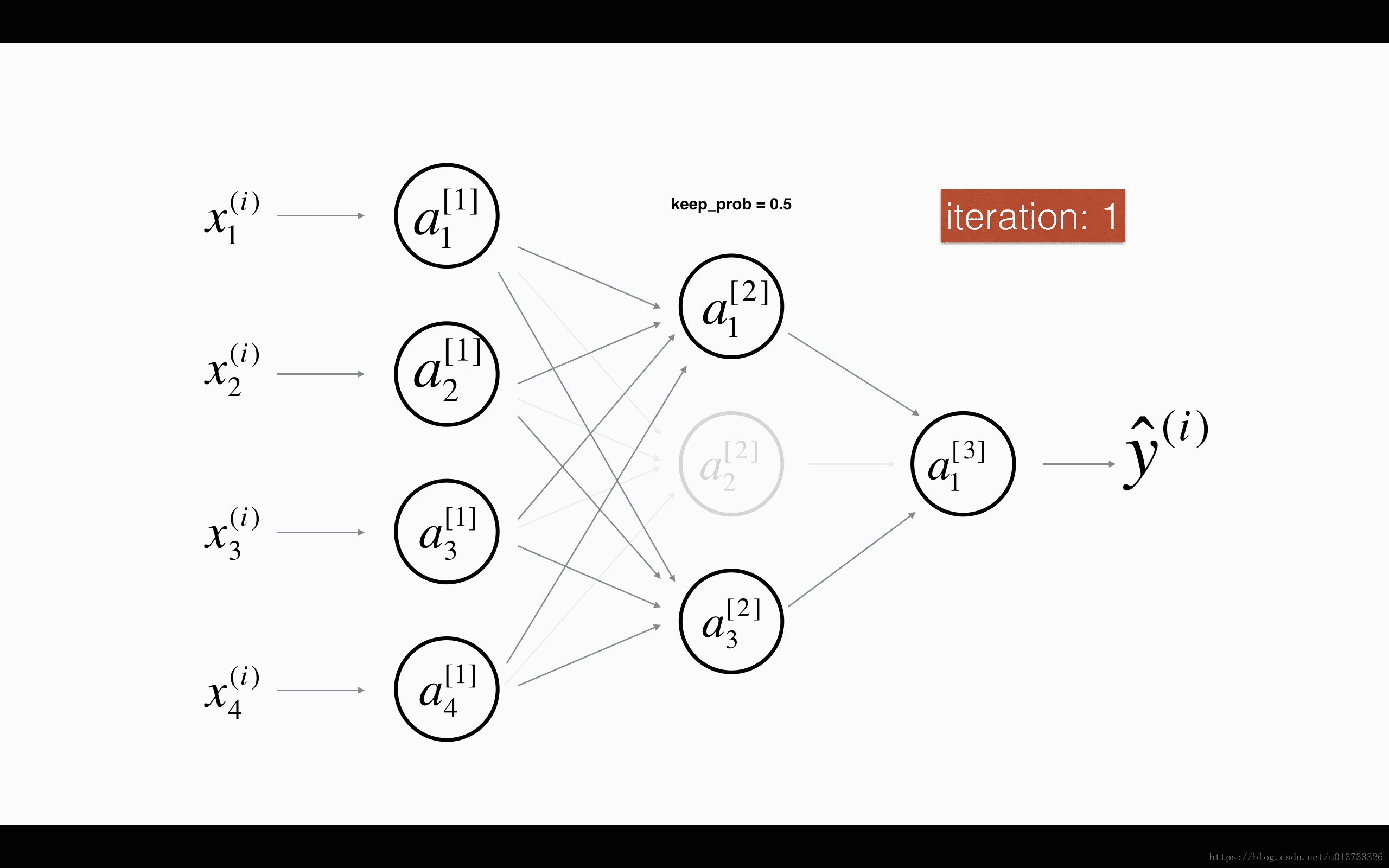
在每一次迭代中,关闭(设置为零)一层的每个神经元,概率为 1−keep_prob1−keep_prob,我们在这里保持概率为keep_probkeep_prob(这里为50%)。丢弃的节点都不参与迭代时的前向和后向传播。
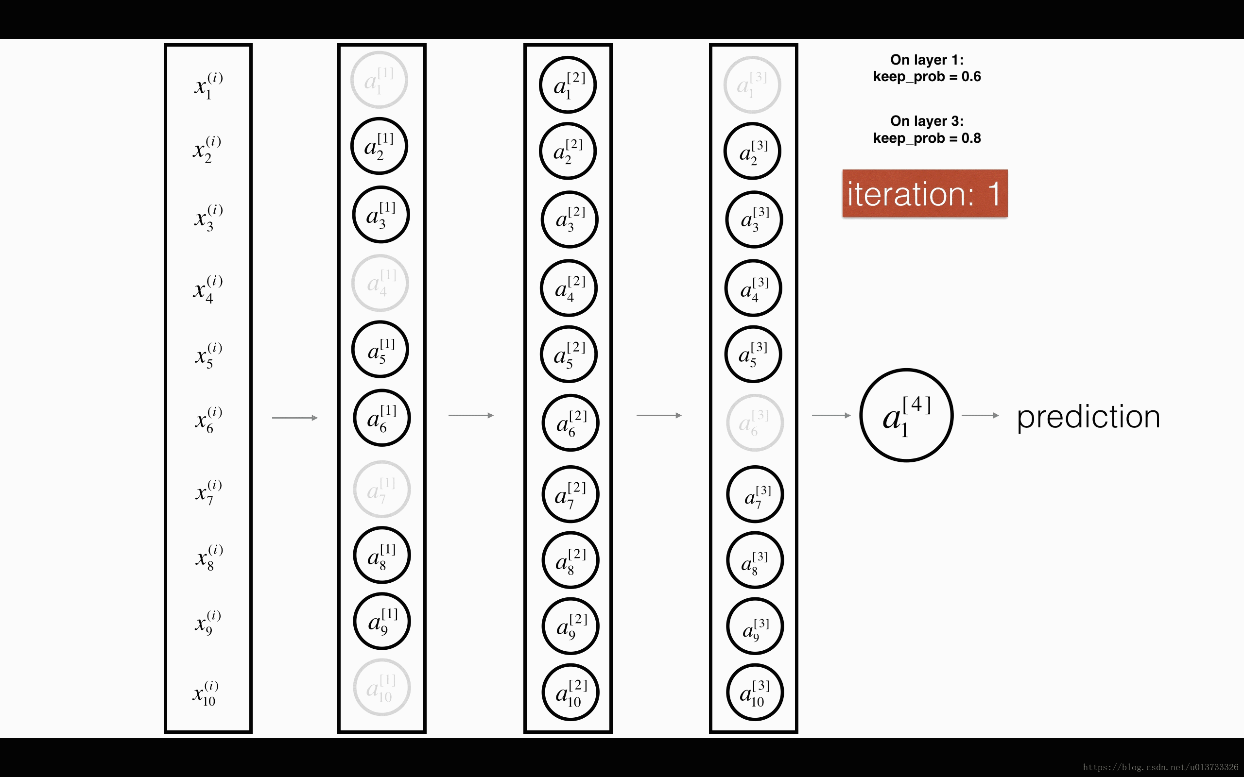
1st1st 平均40%节点被删除, 3rd3rd 平均删除了20%的节点
下面我们将关闭第一层和第三层的一些节点,我们需要做以下四步:
- 在视频中,吴恩达老师讲解了使用
np.random.rand()来初始化和a[1]a[1]具有相同维度的 d[1]d[1] ,在这里,我们将使用向量化实现,我们先来实现一个和A[1]A[1]相同的随机矩阵D[1]=[d[1](1)d[1](2)...d[1](m)]D[1]=[d[1](1)d[1](2)...d[1](m)]。 - 如果D[1]D[1] 低于 (
keep_prob)的值我们就把它设置为0,如果高于(keep_prob)的值我们就设置为1。 - 把A[1]A[1] 更新为 A[1]∗D[1]A[1]∗D[1]。 (我们已经关闭了一些节点)。我们可以使用 D[1]D[1] 作为掩码。我们做矩阵相乘的时候,关闭的那些节点(值为0)就会不参与计算,因为0乘以任何值都为0。
- 使用 A[1]A[1] 除以
keep_prob。这样做的话我们通过缩放就在计算成本的时候仍然具有相同的期望值,这叫做反向dropout。
def forward_propagation_with_dropout(X,parameters,keep_prob=0.5): """ 实现具有随机舍弃节点的前向传播。 LINEAR -> RELU + DROPOUT -> LINEAR -> RELU + DROPOUT -> LINEAR -> SIGMOID. 参数: X - 输入数据集,维度为(2,示例数) parameters - 包含参数“W1”,“b1”,“W2”,“b2”,“W3”,“b3”的python字典: W1 - 权重矩阵,维度为(20,2) b1 - 偏向量,维度为(20,1) W2 - 权重矩阵,维度为(3,20) b2 - 偏向量,维度为(3,1) W3 - 权重矩阵,维度为(1,3) b3 - 偏向量,维度为(1,1) keep_prob - 随机删除的概率,实数 返回: A3 - 最后的激活值,维度为(1,1),正向传播的输出 cache - 存储了一些用于计算反向传播的数值的元组 """ np.random.seed(1) W1 = parameters["W1"] b1 = parameters["b1"] W2 = parameters["W2"] b2 = parameters["b2"] W3 = parameters["W3"] b3 = parameters["b3"] #LINEAR -> RELU -> LINEAR -> RELU -> LINEAR -> SIGMOID Z1 = np.dot(W1,X) + b1 A1 = reg_utils.relu(Z1) #下面的步骤1-4对应于上述的步骤1-4。 D1 = np.random.rand(A1.shape[0],A1.shape[1]) #步骤1:初始化矩阵D1 = np.random.rand(..., ...) D1 = D1 < keep_prob #步骤2:将D1的值转换为0或1(使用keep_prob作为阈值) A1 = A1 * D1 #步骤3:舍弃A1的一些节点(将它的值变为0或False) A1 = A1 / keep_prob #步骤4:缩放未舍弃的节点(不为0)的值 """ #不理解的同学运行一下下面代码就知道了。 import numpy as np np.random.seed(1) A1 = np.random.randn(1,3) D1 = np.random.rand(A1.shape[0],A1.shape[1]) keep_prob=0.5 D1 = D1 < keep_prob print(D1) A1 = 0.01 A1 = A1 * D1 A1 = A1 / keep_prob print(A1) """ Z2 = np.dot(W2,A1) + b2 A2 = reg_utils.relu(Z2) #下面的步骤1-4对应于上述的步骤1-4。 D2 = np.random.rand(A2.shape[0],A2.shape[1]) #步骤1:初始化矩阵D2 = np.random.rand(..., ...) D2 = D2 < keep_prob #步骤2:将D2的值转换为0或1(使用keep_prob作为阈值) A2 = A2 * D2 #步骤3:舍弃A1的一些节点(将它的值变为0或False) A2 = A2 / keep_prob #步骤4:缩放未舍弃的节点(不为0)的值 Z3 = np.dot(W3, A2) + b3 A3 = reg_utils.sigmoid(Z3) cache = (Z1, D1, A1, W1, b1, Z2, D2, A2, W2, b2, Z3, A3, W3, b3) return A3, cache - 1
- 2
- 3
- 4
- 5
- 6
- 7
- 8
- 9
- 10
- 11
- 12
- 13
- 14
- 15
- 16
- 17
- 18
- 19
- 20
- 21
- 22
- 23
- 24
- 25
- 26
- 27
- 28
- 29
- 30
- 31
- 32
- 33
- 34
- 35
- 36
- 37
- 38
- 39
- 40
- 41
- 42
- 43
- 44
- 45
- 46
- 47
- 48
- 49
- 50
- 51
- 52
- 53
- 54
- 55
- 56
- 57
- 58
- 59
- 60
- 61
- 62
- 63
- 64
- 65
- 66
- 67
- 68
- 69
- 70
改变了前向传播的算法,我们也需要改变后向传播的算法,使用存储在缓存中的掩码D[1]D[1] 和 D[2]D[2]将舍弃的节点位置信息添加到第一个和第二个隐藏层。
def backward_propagation_with_dropout(X,Y,cache,keep_prob):
""" 实现我们随机删除的模型的后向传播。 参数: X - 输入数据集,维度为(2,示例数) Y - 标签,维度为(输出节点数量,示例数量) cache - 来自forward_propagation_with_dropout()的cache输出 keep_prob - 随机删除的概率,实数 返回: gradients - 一个关于每个参数、激活值和预激活变量的梯度值的字典 """ m = X.shape[1] (Z1, D1, A1, W1, b1, Z2, D2, A2, W2, b2, Z3, A3, W3, b3) = cache dZ3 = A3 - Y dW3 = (1 / m) * np.dot(dZ3,A2.T) db3 = 1. / m * np.sum(dZ3, axis=1, keepdims=True) dA2 = np.dot(W3.T, dZ3) dA2 = dA2 * D2 # 步骤1:使用正向传播期间相同的节点,舍弃那些关闭的节点(因为任何数乘以0或者False都为0或者False) dA2 = dA2 / keep_prob # 步骤2:缩放未舍弃的节点(不为0)的值 dZ2 = np.multiply(dA2, np.int64(A2 > 0)) dW2 = 1. / m * np.dot(dZ2, A1.T) db2 = 1. / m * np.sum(dZ2, axis=1, keepdims=True) dA1 = np.dot(W2.T, dZ2) dA1 = dA1 * D1 # 步骤1:使用正向传播期间相同的节点,舍弃那些关闭的节点(因为任何数乘以0或者False都为0或者False) dA1 = dA1 / keep_prob # 步骤2:缩放未舍弃的节点(不为0)的值 dZ1 = np.multiply(dA1, np.int64(A1 > 0)) dW1 = 1. / m * np.dot(dZ1, X.T) db1 = 1. / m * np.sum(dZ1, axis=1, keepdims=True) gradients = {"dZ3": dZ3, "dW3": dW3, "db3": db3,"dA2": dA2, "dZ2": dZ2, "dW2": dW2, "db2": db2, "dA1": dA1, "dZ1": dZ1, "dW1": dW1, "db1": db1} return gradients- 1
- 2
- 3
- 4
- 5
- 6
- 7
- 8
- 9
- 10
- 11
- 12
- 13
- 14
- 15
- 16
- 17
- 18
- 19
- 20
- 21
- 22
- 23
- 24
- 25
- 26
- 27
- 28
- 29
- 30
- 31
- 32
- 33
- 34
- 35
- 36
- 37
- 38
- 39
- 40
- 41
我们前向和后向传播的函数都写好了,现在用dropout运行模型(keep_prob = 0.86)跑一波。这意味着在每次迭代中,程序都可以24%的概率关闭第1层和第2层的每个神经元。调用的时候:
- 使用forward_propagation_with_dropout而不是forward_propagation。
- 使用backward_propagation_with_dropout而不是backward_propagation。
parameters = model(train_X, train_Y, keep_prob=0.86, learning_rate=0.3,is_plot=True)

print("使用随机删除节点,训练集:")
predictions_train = reg_utils.predict(train_X, train_Y, parameters)
print("使用随机删除节点,测试集:") reg_utils.predictions_test = reg_utils.predict(test_X, test_Y, parameters)- 1
- 2
- 3
- 4
- 5
- 6
执行结果:
第0次迭代,成本值为:0.654391240515
第10000次迭代,成本值为:0.0610169865749
第20000次迭代,成本值为:0.0605824357985 使用随机删除节点,训练集: Accuracy: 0.928909952607 使用随机删除节点,测试集: Accuracy: 0.95- 1
- 2
- 3
- 4
- 5
- 6
- 7
- 8
我们来看看它的分类情况:
plt.title("Model with dropout")
axes = plt.gca()
axes.set_xlim([-0.75, 0.40]) axes.set_ylim([-0.75, 0.65]) reg_utils.plot_decision_boundary(lambda x: reg_utils.predict_dec(parameters, x.T), train_X, train_Y)- 1
- 2
- 3
- 4
- 5
执行结果:
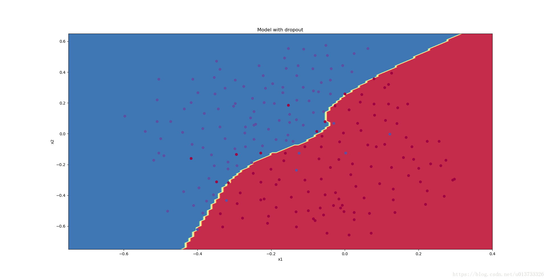
我们可以看到,正则化会把训练集的准确度降低,但是测试集的准确度提高了,所以,我们这个还是成功了。