P0 前言
- 第二门课 : Improving Deep Neural Networks: Hyperparameter turing,Regularization and Optimization (改善深层神经网络:超参数调试、正则化以及优化)
- 第二周 : Optimization algorithms (优化算法)
- 主要知识点 : Mini-batch梯度下降、指数加权平均、Momentum梯度下降、RMSprop、Adam优化算法、衰减学习率、局部最优等;
视频地址 : https://mooc.study.163.com/course/2001281003#/info
笔记地址:
数据集,源码,作业的本地版网页缓存下载:链接:https://pan.baidu.com/s/1yIVXHmyRxrUQMFfulQPXYQ 提取码:k544
P1 作业
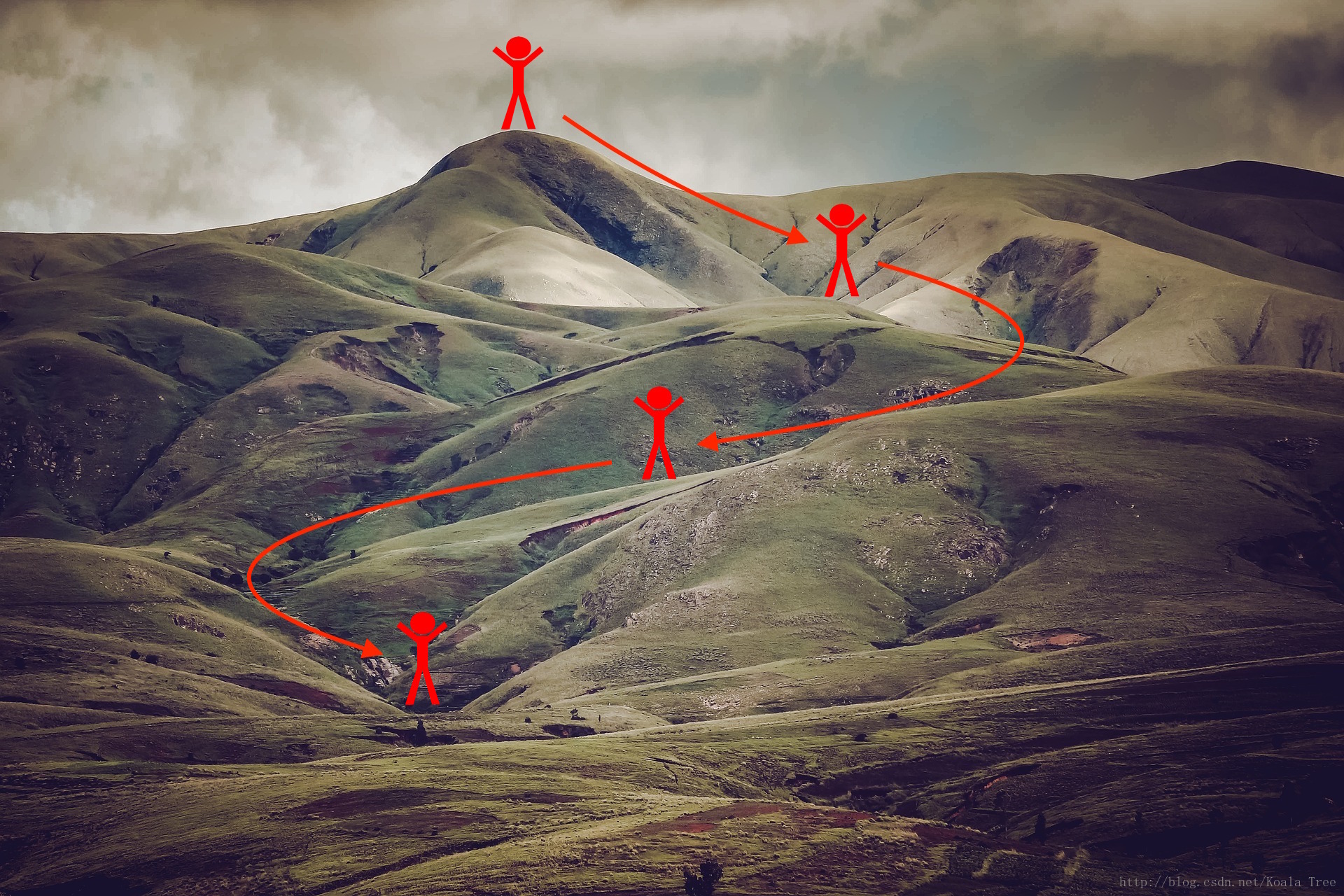
梯度下降过程类比:
需要的包:
import numpy as np
import matplotlib.pyplot as plt
import scipy.io
import math
import sklearn
import sklearn.datasets

from opt_utils import load_params_and_grads, initialize_parameters, forward_propagation, backward_propagation
from opt_utils import compute_cost, predict, predict_dec, plot_decision_boundary, load_dataset
from testCases import *

%matplotlib inline
plt.rcParams['figure.figsize'] = (7.0, 4.0) # set default size of plots
plt.rcParams['image.interpolation'] = 'nearest'
plt.rcParams['image.cmap'] = 'gray'
有用的函数:
def load_params_and_grads(seed=1):
np.random.seed(seed)
W1 = np.random.randn(2,3)
b1 = np.random.randn(2,1)
W2 = np.random.randn(3,3)
b2 = np.random.randn(3,1)
dW1 = np.random.randn(2,3)
db1 = np.random.randn(2,1)
dW2 = np.random.randn(3,3)
db2 = np.random.randn(3,1)
return W1, b1, W2, b2, dW1, db1, dW2, db2
def initialize_parameters(layer_dims):
"""
Arguments:
layer_dims -- python array (list) containing the dimensions of each layer in our network
Returns:
parameters -- python dictionary containing your parameters "W1", "b1", ..., "WL", "bL":
W1 -- weight matrix of shape (layer_dims[l], layer_dims[l-1])
b1 -- bias vector of shape (layer_dims[l], 1)
Wl -- weight matrix of shape (layer_dims[l-1], layer_dims[l])
bl -- bias vector of shape (1, layer_dims[l])
Tips:
- For example: the layer_dims for the "Planar Data classification model" would have been [2,2,1].
This means W1's shape was (2,2), b1 was (1,2), W2 was (2,1) and b2 was (1,1). Now you have to generalize it!
- In the for loop, use parameters['W' + str(l)] to access Wl, where l is the iterative integer.
"""
np.random.seed(3)
parameters = {}
L = len(layer_dims) # number of layers in the network
for l in range(1, L):
parameters['W' + str(l)] = np.random.randn(layer_dims[l], layer_dims[l-1])* np.sqrt(2 / layer_dims[l-1])
parameters['b' + str(l)] = np.zeros((layer_dims[l], 1))
assert(parameters['W' + str(l)].shape == layer_dims[l], layer_dims[l-1])
assert(parameters['W' + str(l)].shape == layer_dims[l], 1)
return parameters
def forward_propagation(X, parameters):
"""
Implements the forward propagation (and computes the loss) presented in Figure 2.
Arguments:
X -- input dataset, of shape (input size, number of examples)
parameters -- python dictionary containing your parameters "W1", "b1", "W2", "b2", "W3", "b3":
W1 -- weight matrix of shape ()
b1 -- bias vector of shape ()
W2 -- weight matrix of shape ()
b2 -- bias vector of shape ()
W3 -- weight matrix of shape ()
b3 -- bias vector of shape ()
Returns:
loss -- the loss function (vanilla logistic loss)
"""
# retrieve parameters
W1 = parameters["W1"]
b1 = parameters["b1"]
W2 = parameters["W2"]
b2 = parameters["b2"]
W3 = parameters["W3"]
b3 = parameters["b3"]
# LINEAR -> RELU -> LINEAR -> RELU -> LINEAR -> SIGMOID
z1 = np.dot(W1, X) + b1
a1 = relu(z1)
z2 = np.dot(W2, a1) + b2
a2 = relu(z2)
z3 = np.dot(W3, a2) + b3
a3 = sigmoid(z3)
cache = (z1, a1, W1, b1, z2, a2, W2, b2, z3, a3, W3, b3)
return a3, cache
def backward_propagation(X, Y, cache):
"""
Implement the backward propagation presented in figure 2.
Arguments:
X -- input dataset, of shape (input size, number of examples)
Y -- true "label" vector (containing 0 if cat, 1 if non-cat)
cache -- cache output from forward_propagation()
Returns:
gradients -- A dictionary with the gradients with respect to each parameter, activation and pre-activation variables
"""
m = X.shape[1]
(z1, a1, W1, b1, z2, a2, W2, b2, z3, a3, W3, b3) = cache
dz3 = 1./m * (a3 - Y)
dW3 = np.dot(dz3, a2.T)
db3 = np.sum(dz3, axis=1, keepdims = True)
da2 = np.dot(W3.T, dz3)
dz2 = np.multiply(da2, np.int64(a2 > 0))
dW2 = np.dot(dz2, a1.T)
db2 = np.sum(dz2, axis=1, keepdims = True)
da1 = np.dot(W2.T, dz2)
dz1 = np.multiply(da1, np.int64(a1 > 0))
dW1 = np.dot(dz1, X.T)
db1 = np.sum(dz1, axis=1, keepdims = True)
gradients = {"dz3": dz3, "dW3": dW3, "db3": db3,
"da2": da2, "dz2": dz2, "dW2": dW2, "db2": db2,
"da1": da1, "dz1": dz1, "dW1": dW1, "db1": db1}
return gradients
def compute_cost(a3, Y):
"""
Implement the cost function
Arguments:
a3 -- post-activation, output of forward propagation
Y -- "true" labels vector, same shape as a3
Returns:
cost - value of the cost function
"""
m = Y.shape[1]
logprobs = np.multiply(-np.log(a3),Y) + np.multiply(-np.log(1 - a3), 1 - Y)
cost = 1./m * np.sum(logprobs)
return cost
def predict(X, y, parameters):
"""
This function is used to predict the results of a n-layer neural network.
Arguments:
X -- data set of examples you would like to label
parameters -- parameters of the trained model
Returns:
p -- predictions for the given dataset X
"""
m = X.shape[1]
p = np.zeros((1,m), dtype = np.int)
# Forward propagation
a3, caches = forward_propagation(X, parameters)
# convert probas to 0/1 predictions
for i in range(0, a3.shape[1]):
if a3[0,i] > 0.5:
p[0,i] = 1
else:
p[0,i] = 0
# print results
#print ("predictions: " + str(p[0,:]))
#print ("true labels: " + str(y[0,:]))
print("Accuracy: " + str(np.mean((p[0,:] == y[0,:]))))
return p
def predict_dec(parameters, X):
"""
Used for plotting decision boundary.
Arguments:
parameters -- python dictionary containing your parameters
X -- input data of size (m, K)
Returns
predictions -- vector of predictions of our model (red: 0 / blue: 1)
"""
# Predict using forward propagation and a classification threshold of 0.5
a3, cache = forward_propagation(X, parameters)
predictions = (a3 > 0.5)
return predictions
def plot_decision_boundary(model, X, y):
# Set min and max values and give it some padding
x_min, x_max = X[0, :].min() - 1, X[0, :].max() + 1
y_min, y_max = X[1, :].min() - 1, X[1, :].max() + 1
h = 0.01
# Generate a grid of points with distance h between them
xx, yy = np.meshgrid(np.arange(x_min, x_max, h), np.arange(y_min, y_max, h))
# Predict the function value for the whole grid
Z = model(np.c_[xx.ravel(), yy.ravel()])
Z = Z.reshape(xx.shape)
# Plot the contour and training examples
plt.contourf(xx, yy, Z, cmap=plt.cm.Spectral)
plt.ylabel('x2')
plt.xlabel('x1')
plt.scatter(X[0, :], X[1, :], c=y, cmap=plt.cm.Spectral)
plt.show()
def load_dataset():
np.random.seed(3)
train_X, train_Y = sklearn.datasets.make_moons(n_samples=300, noise=.2) #300 #0.2
# Visualize the data
plt.scatter(train_X[:, 0], train_X[:, 1], c=train_Y, s=40, cmap=plt.cm.Spectral);
train_X = train_X.T
train_Y = train_Y.reshape((1, train_Y.shape[0]))
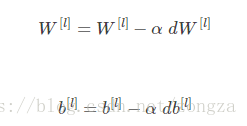
return train_X, train_Y1-梯度下降
公式如下:
# GRADED FUNCTION: update_parameters_with_gd

def update_parameters_with_gd(parameters, grads, learning_rate):
    """
    Update parameters using one step of gradient descent

    Arguments:
    parameters -- python dictionary containing your parameters to be updated:
                    parameters['W' + str(l)] = Wl
                    parameters['b' + str(l)] = bl
    grads -- python dictionary containing your gradients to update each parameters:
                    grads['dW' + str(l)] = dWl
                    grads['db' + str(l)] = dbl
    learning_rate -- the learning rate, scalar.

    Returns:
    parameters -- python dictionary containing your updated parameters
    """

    L = len(parameters) // 2 # number of layers in the neural networks

    # Update rule for each parameter
    for l in range(L):
        ### START CODE HERE ### (approx. 2 lines)
        parameters["W" + str(l+1)] = parameters["W" + str(l+1)] - learning_rate*grads["dW" + str(l+1)]
        parameters["b" + str(l+1)] = parameters["b" + str(l+1)] - learning_rate*grads["db" + str(l+1)]
        ### END CODE HERE ###

    return parameters
parameters, grads, learning_rate = update_parameters_with_gd_test_case()
parameters = update_parameters_with_gd(parameters, grads, learning_rate)
print("W1 = " + str(parameters["W1"]))
print("b1 = " + str(parameters["b1"]))
print("W2 = " + str(parameters["W2"]))
print("b2 = " + str(parameters["b2"]))
#结果
W1 = [[ 1.63535156 -0.62320365 -0.53718766]
[-1.07799357 0.85639907 -2.29470142]]
b1 = [[ 1.74604067]
[-0.75184921]]
W2 = [[ 0.32171798 -0.25467393 1.46902454]
[-2.05617317 -0.31554548 -0.3756023 ]
[ 1.1404819 -1.09976462 -0.1612551 ]]
b2 = [[-0.88020257]
[ 0.02561572]
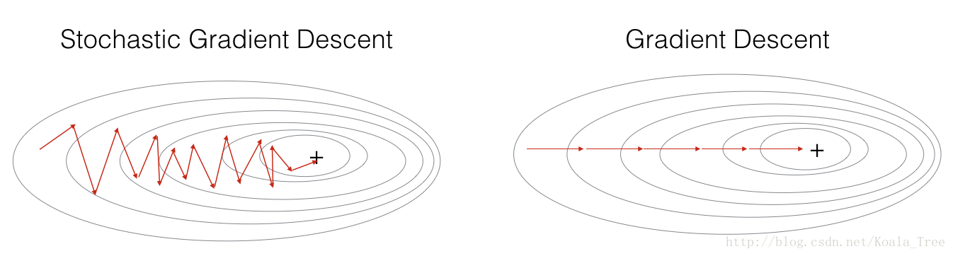
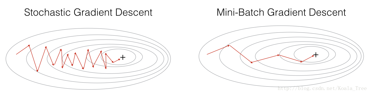
[ 0.57539477]]这种方法的一个变体是随机梯度下降法(SGD),它相当于小批梯度下降法,其中每个小批只有一个示例。您刚刚实现的更新规则不会改变。改变的是你一次只计算一个训练例子的梯度,而不是整个训练集。下面的代码例子说明了随机梯度下降和(批量)梯度下降的区别。
- (Batch) Gradient Descent:
X = data_input
Y = labels
parameters = initialize_parameters(layers_dims)
for i in range(0, num_iterations):
    # Forward propagation
    a, caches = forward_propagation(X, parameters)
    # Compute cost.
    cost = compute_cost(a, Y)
    # Backward propagation.
    grads = backward_propagation(a, caches, parameters)
    # Update parameters.
    parameters = update_parameters(parameters, grads)
- Stochastic Gradient Descent:
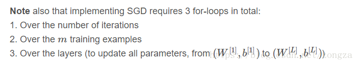
X = data_input
Y = labels
parameters = initialize_parameters(layers_dims)
for i in range(0, num_iterations):
    for j in range(0, m):
        # Forward propagation
        a, caches = forward_propagation(X[:,j], parameters)
        # Compute cost
        cost = compute_cost(a, Y[:,j])
        # Backward propagation
        grads = backward_propagation(a, caches, parameters)
        # Update parameters.
        parameters = update_parameters(parameters, grads)
在随机梯度下降法中,在更新梯度之前只使用一个训练示例。当训练集较大时,SGD可以更快。但这些参数将“振荡”到最小值,而不是平稳地收敛。下面是一个例子:
在实践中,通常使用mini_batch的梯度下降,他相比GD和SGD的区别在于你用来执行一个更新步骤的例子数量(MGD在两者中间)。为此你需要调一个超参数alpha。
2 - Mini-Batch Gradient descent
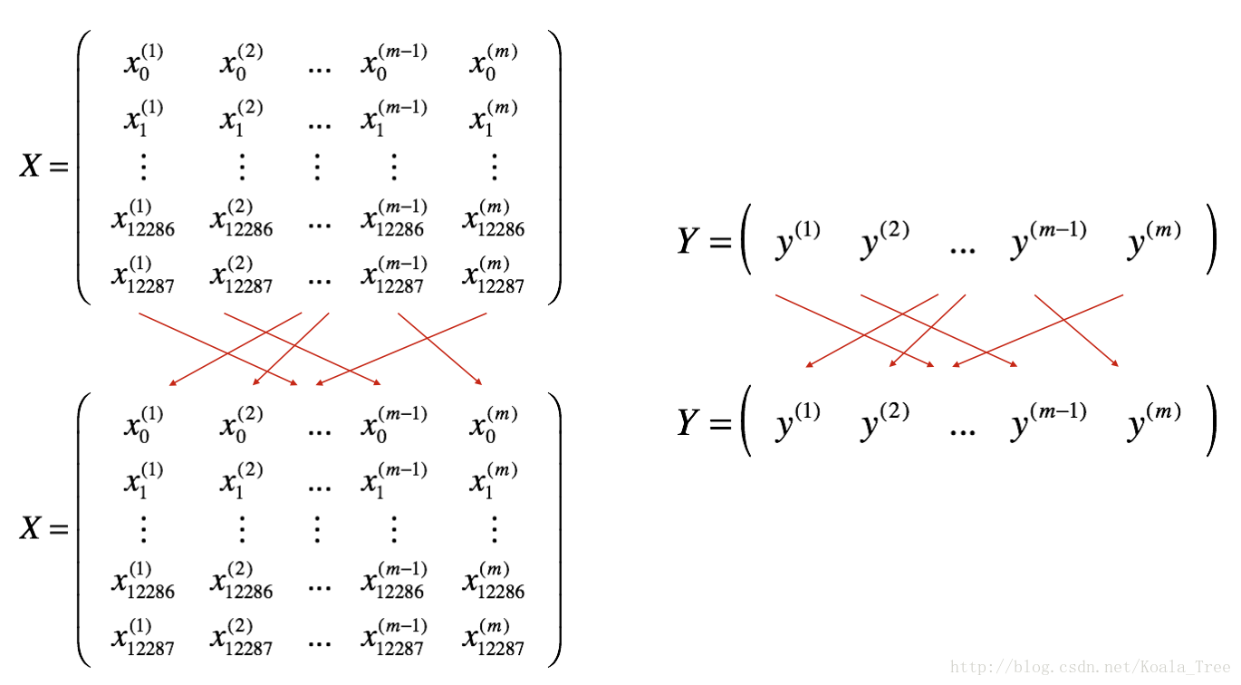
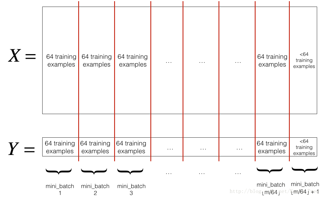
主要有两步:打乱(Shuffle)和分区(Partition)
Shuffle图解:
Partition图解 :

def random_mini_batches(X, Y, mini_batch_size=64, seed=0):
    """
    Creates a list of random minibatches from (X, Y)

    Arguments:
    X -- input data, of shape (input size, number of examples)
    Y -- true "label" vector (1 for blue dot / 0 for red dot), of shape (1, number of examples)
    mini_batch_size -- size of the mini-batches, integer

    Returns:
    mini_batches -- list of synchronous (mini_batch_X, mini_batch_Y)
    """

    np.random.seed(seed)  # To make your "random" minibatches the same as ours
    m = X.shape[1]  # number of training examples
    mini_batches = []

    # Step 1: Shuffle (X, Y)
    permutation = list(np.random.permutation(m))
    shuffled_X = X[:, permutation]
    shuffled_Y = Y[:, permutation].reshape((1, m))


    # Step 2: Partition (shuffled_X, shuffled_Y). Minus the end case.
    num_complete_minibatches = int(math.floor( 1.* m / mini_batch_size)) #ng这里没有强制转换会报错 # number of mini batches of size mini_batch_size in your partitionning
    for k in range(0,num_complete_minibatches):
        ### START CODE HERE ### (approx. 2 lines)
        mini_batch_X = shuffled_X[:, (k)*mini_batch_size : (k+1)*mini_batch_size]#刚开始(k+1)*mini_batch_size-1了,实际上切片包括起点但不包括终点!!
        mini_batch_Y = shuffled_Y[:, (k)*mini_batch_size : (k+1)*mini_batch_size]
        ### END CODE HERE ###
        mini_batch = (mini_batch_X, mini_batch_Y)
        mini_batches.append(mini_batch)

    # Handling the end case (last mini-batch < mini_batch_size)
    if m % mini_batch_size != 0:
        ### START CODE HERE ### (approx. 2 lines)
        mini_batch_X = shuffled_X[:, (num_complete_minibatches)*mini_batch_size : m]
        mini_batch_Y = shuffled_Y[:, (num_complete_minibatches)*mini_batch_size : m]
        ### END CODE HERE ###
        mini_batch = (mini_batch_X, mini_batch_Y)
        mini_batches.append(mini_batch)

    return mini_batches
X_assess, Y_assess, mini_batch_size = random_mini_batches_test_case()
mini_batches = random_mini_batches(X_assess, Y_assess, mini_batch_size)
print ("shape of the 1st mini_batch_X: " + str(mini_batches[0][0].shape))
print ("shape of the 2nd mini_batch_X: " + str(mini_batches[1][0].shape))
print ("shape of the 3rd mini_batch_X: " + str(mini_batches[2][0].shape))
print ("shape of the 1st mini_batch_Y: " + str(mini_batches[0][1].shape))
print ("shape of the 2nd mini_batch_Y: " + str(mini_batches[1][1].shape))
print ("shape of the 3rd mini_batch_Y: " + str(mini_batches[2][1].shape))
print ("mini batch sanity check: " + str(mini_batches[0][0][0][0:3]))
#结果
shape of the 1st mini_batch_X: (12288, 64)
shape of the 2nd mini_batch_X: (12288, 64)
shape of the 3rd mini_batch_X: (12288, 20)
shape of the 1st mini_batch_Y: (1, 64)
shape of the 2nd mini_batch_Y: (1, 64)
shape of the 3rd mini_batch_Y: (1, 20)
mini batch sanity check: [ 0.90085595 -0.7612069 0.2344157 ]总结:
- batch的大小通常选2的倍数e.g., 16, 32, 64, 128.
3 - Momentum
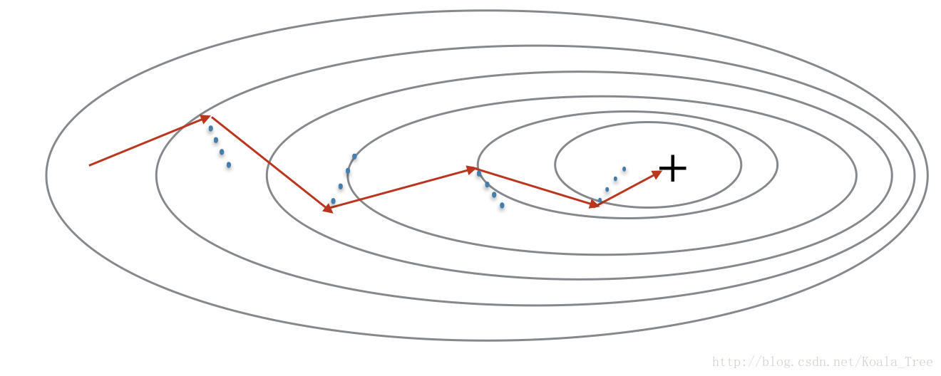
MGD仍然存在震荡(因为每次只用一部分样本来更新参数),因此才有了冲量方法,他可以缓解这个问题。
动量方法会考虑过去的梯度来使得更新更平滑。我们将在变量v中存储之前梯度的“方向”。形式上,这是梯度的指数加权平均值。你也可以把v看作是滚落的球的“速度”,根据山坡的坡度/坡度的方向来增加速度(和动量)。
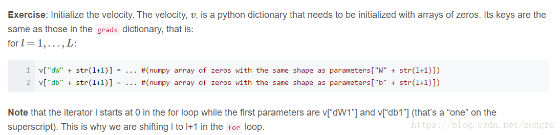
# GRADED FUNCTION: initialize_velocity

def initialize_velocity(parameters):
    """
    Initializes the velocity as a python dictionary with:
                - keys: "dW1", "db1", ..., "dWL", "dbL"
                - values: numpy arrays of zeros of the same shape as the corresponding gradients/parameters.
    Arguments:
    parameters -- python dictionary containing your parameters.
                    parameters['W' + str(l)] = Wl
                    parameters['b' + str(l)] = bl

    Returns:
    v -- python dictionary containing the current velocity.
                    v['dW' + str(l)] = velocity of dWl
                    v['db' + str(l)] = velocity of dbl
    """

    L = len(parameters) // 2 # number of layers in the neural networks
    v = {}

    # Initialize velocity
    for l in range(L):
        ### START CODE HERE ### (approx. 2 lines)
        v["dW" + str(l+1)] = np.zeros(parameters["W" + str(l+1)].shape)
        v["db" + str(l+1)] = np.zeros(parameters["b" + str(l+1)].shape)
        ### END CODE HERE ###

    return v
parameters = initialize_velocity_test_case()
v = initialize_velocity(parameters)
print("v[\"dW1\"] = " + str(v["dW1"]))
print("v[\"db1\"] = " + str(v["db1"]))
print("v[\"dW2\"] = " + str(v["dW2"]))
print("v[\"db2\"] = " + str(v["db2"]))
#下面是结果
v["dW1"] = [[ 0. 0. 0.]
[ 0. 0. 0.]]
v["db1"] = [[ 0.]
[ 0.]]
v["dW2"] = [[ 0. 0. 0.]
[ 0. 0. 0.]
[ 0. 0. 0.]]
v["db2"] = [[ 0.]
[ 0.]
[ 0.]]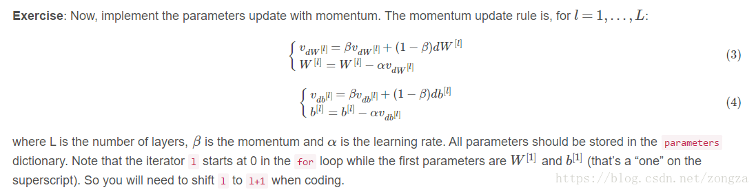
def update_parameters_with_momentum(parameters, grads, v, beta, learning_rate):
    """
    Update parameters using Momentum

    Arguments:
    parameters -- python dictionary containing your parameters:
                    parameters['W' + str(l)] = Wl
                    parameters['b' + str(l)] = bl
    grads -- python dictionary containing your gradients for each parameters:
                    grads['dW' + str(l)] = dWl
                    grads['db' + str(l)] = dbl
    v -- python dictionary containing the current velocity:
                    v['dW' + str(l)] = ...
                    v['db' + str(l)] = ...
    beta -- the momentum hyperparameter, scalar
    learning_rate -- the learning rate, scalar

    Returns:
    parameters -- python dictionary containing your updated parameters
    v -- python dictionary containing your updated velocities
    """

    L = len(parameters) // 2  # number of layers in the neural networks

    # Momentum update for each parameter
    for l in range(L):
        ### START CODE HERE ### (approx. 4 lines)
        # compute velocities
        v["dW" + str(l + 1)] = beta*v["dW" + str(l + 1)] +(1 - beta)*grads["dW"+str(l + 1)]#beta相当于考虑之前的梯度影响的比例
        v["db" + str(l + 1)] = beta*v["db" + str(l + 1)] +(1 - beta)*grads["db"+str(l + 1)]
        # update parameters
        parameters["W" + str(l + 1)] -= learning_rate*v["dW" + str(l + 1)]
        parameters["b" + str(l + 1)] -= learning_rate*v["db" + str(l + 1)]
        ### END CODE HERE ###

    return parameters, v
parameters, grads, v = update_parameters_with_momentum_test_case()
parameters, v = update_parameters_with_momentum(parameters, grads, v, beta = 0.9, learning_rate = 0.01)
print("W1 = " + str(parameters["W1"]))
print("b1 = " + str(parameters["b1"]))
print("W2 = " + str(parameters["W2"]))
print("b2 = " + str(parameters["b2"]))
print("v[\"dW1\"] = " + str(v["dW1"]))
print("v[\"db1\"] = " + str(v["db1"]))
print("v[\"dW2\"] = " + str(v["dW2"]))
print("v[\"db2\"] = " + str(v["db2"]))
#结果
W1 = [[ 1.62544598 -0.61290114 -0.52907334]
[-1.07347112 0.86450677 -2.30085497]]
b1 = [[ 1.74493465]
[-0.76027113]]
W2 = [[ 0.31930698 -0.24990073 1.4627996 ]
[-2.05974396 -0.32173003 -0.38320915]
[ 1.13444069 -1.0998786 -0.1713109 ]]
b2 = [[-0.87809283]
[ 0.04055394]
[ 0.58207317]]
v["dW1"] = [[-0.11006192 0.11447237 0.09015907]
[ 0.05024943 0.09008559 -0.06837279]]
v["db1"] = [[-0.01228902]
[-0.09357694]]
v["dW2"] = [[-0.02678881 0.05303555 -0.06916608]
[-0.03967535 -0.06871727 -0.08452056]
[-0.06712461 -0.00126646 -0.11173103]]
v["db2"] = [[ 0.02344157]
[ 0.16598022]
[ 0.07420442]]注意:
- v被初始化为0,因此需要迭代几次才能正常工作
- 如果beta=0,则M退化为标准的GD
如何选择beta?
- beta越大,更新越平滑,但是同时也会削弱很多更新效果
- 一般beta都在0.8-0.999,大家都选的0.9作为默认值
- beta是个超参,你需要微调他,选择能使J最小的那个值
总结:
- 动量把过去的梯度考虑在内,以平滑梯度下降的步骤。适用于批量梯度下降法、小批量梯度下降法或随机梯度下降法
- M方法有两个超参数:alpha和beta
4 - Adam
A相当于在M的基础上又增加了一个平方版本的冲量信息,利用原来的冲量信息和现在的平方版冲量信息联合决策更新。
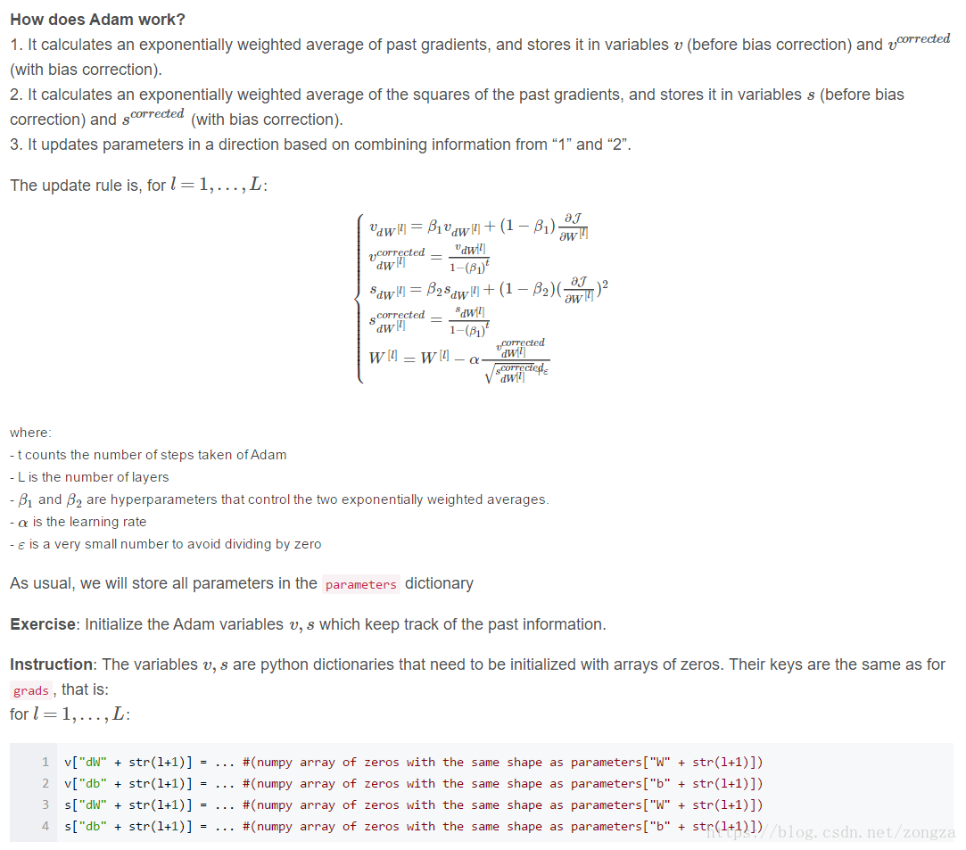
# GRADED FUNCTION: initialize_adam

def initialize_adam(parameters) :
    """
    Initializes v and s as two python dictionaries with:
                - keys: "dW1", "db1", ..., "dWL", "dbL"
                - values: numpy arrays of zeros of the same shape as the corresponding gradients/parameters.

    Arguments:
    parameters -- python dictionary containing your parameters.
                    parameters["W" + str(l)] = Wl
                    parameters["b" + str(l)] = bl

    Returns:
    v -- python dictionary that will contain the exponentially weighted average of the gradient.
                    v["dW" + str(l)] = ...
                    v["db" + str(l)] = ...
    s -- python dictionary that will contain the exponentially weighted average of the squared gradient.
                    s["dW" + str(l)] = ...
                    s["db" + str(l)] = ...

    """

    L = len(parameters) // 2 # number of layers in the neural networks
    v = {}
    s = {}

    # Initialize v, s. Input: "parameters". Outputs: "v, s".
    for l in range(L):
    ### START CODE HERE ### (approx. 4 lines)
        v["dW" + str(l+1)] = np.zeros(parameters["W" + str(l+1)].shape)
        v["db" + str(l+1)] = np.zeros(parameters["b" + str(l+1)].shape)
        s["dW" + str(l+1)] = np.zeros(parameters["W" + str(l+1)].shape)
        s["db" + str(l+1)] = np.zeros(parameters["b" + str(l+1)].shape)
    ### END CODE HERE ###

    return v, s
parameters = initialize_adam_test_case()
v, s = initialize_adam(parameters)
print("v[\"dW1\"] = " + str(v["dW1"]))
print("v[\"db1\"] = " + str(v["db1"]))
print("v[\"dW2\"] = " + str(v["dW2"]))
print("v[\"db2\"] = " + str(v["db2"]))
print("s[\"dW1\"] = " + str(s["dW1"]))
print("s[\"db1\"] = " + str(s["db1"]))
print("s[\"dW2\"] = " + str(s["dW2"]))
print("s[\"db2\"] = " + str(s["db2"]))
#结果:
v["dW1"] = [[ 0. 0. 0.]
[ 0. 0. 0.]]
v["db1"] = [[ 0.]
[ 0.]]
v["dW2"] = [[ 0. 0. 0.]
[ 0. 0. 0.]
[ 0. 0. 0.]]
v["db2"] = [[ 0.]
[ 0.]
[ 0.]]
s["dW1"] = [[ 0. 0. 0.]
[ 0. 0. 0.]]
s["db1"] = [[ 0.]
[ 0.]]
s["dW2"] = [[ 0. 0. 0.]
[ 0. 0. 0.]
[ 0. 0. 0.]]
s["db2"] = [[ 0.]
[ 0.]
[ 0.]]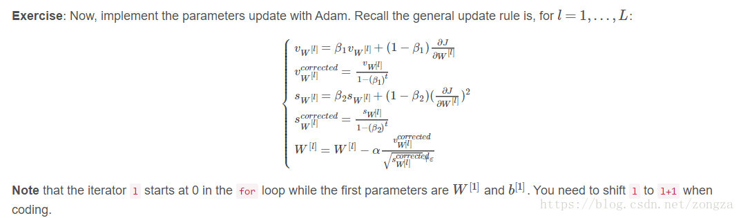
def update_parameters_with_adam(parameters, grads, v, s, t, learning_rate=0.01,
beta1=0.9, beta2=0.999, epsilon=1e-8):
"""
Update parameters using Adam
Arguments:
parameters -- python dictionary containing your parameters:
parameters['W' + str(l)] = Wl
parameters['b' + str(l)] = bl
grads -- python dictionary containing your gradients for each parameters:
grads['dW' + str(l)] = dWl
grads['db' + str(l)] = dbl
v -- Adam variable, moving average of the first gradient, python dictionary
s -- Adam variable, moving average of the squared gradient, python dictionary
learning_rate -- the learning rate, scalar.
beta1 -- Exponential decay hyperparameter for the first moment estimates
beta2 -- Exponential decay hyperparameter for the second moment estimates
epsilon -- hyperparameter preventing division by zero in Adam updates
Returns:
parameters -- python dictionary containing your updated parameters
v -- Adam variable, moving average of the first gradient, python dictionary
s -- Adam variable, moving average of the squared gradient, python dictionary
"""
L = len(parameters) // 2 # number of layers in the neural networks
v_corrected = {} # Initializing first moment estimate, python dictionary
s_corrected = {} # Initializing second moment estimate, python dictionary
# Perform Adam update on all parameters
for l in range(L):
# Moving average of the gradients. Inputs: "v, grads, beta1". Output: "v".
### START CODE HERE ### (approx. 2 lines)
v["dW" + str(l + 1)] = beta1*v["dW" + str(l + 1)] +(1 - beta1)*grads["dW"+str(l + 1)]
v["db" + str(l + 1)] = beta1*v["db" + str(l + 1)] +(1 - beta1)*grads["db"+str(l + 1)]
### END CODE HERE ###
# Compute bias-corrected first moment estimate. Inputs: "v, beta1, t". Output: "v_corrected".
### START CODE HERE ### (approx. 2 lines)
v_corrected["dW" + str(l + 1)] = v["dW" + str(l + 1)]/(1-beta1)
v_corrected["db" + str(l + 1)] = v["db" + str(l + 1)]/(1-beta1)
### END CODE HERE ###
# Moving average of the squared gradients. Inputs: "s, grads, beta2". Output: "s".
### START CODE HERE ### (approx. 2 lines)
s["dW" + str(l + 1)] = beta2*s["dW" + str(l + 1)] +(1 - beta2) * grads["dW"+str(l + 1)]**2
s["db" + str(l + 1)] = beta2*s["db" + str(l + 1)] +(1 - beta2) * grads["db"+str(l + 1)]**2
### END CODE HERE ###
# Compute bias-corrected second raw moment estimate. Inputs: "s, beta2, t". Output: "s_corrected".
### START CODE HERE ### (approx. 2 lines)
s_corrected["dW" + str(l + 1)] = s["dW" + str(l + 1)]/(1-beta2)
s_corrected["db" + str(l + 1)] = s["db" + str(l + 1)]/(1-beta2)
### END CODE HERE ###
# Update parameters. Inputs: "parameters, learning_rate, v_corrected, s_corrected, epsilon". Output: "parameters".
### START CODE HERE ### (approx. 2 lines)
parameters["W" + str(l + 1)] -= learning_rate * v_corrected["dW" + str(l + 1)]/(np.sqrt(s_corrected["dW" + str(l + 1)])+epsilon)
parameters["b" + str(l + 1)] -= learning_rate * v_corrected["db" + str(l + 1)]/(np.sqrt(s_corrected["db" + str(l + 1)])+epsilon)
### END CODE HERE ###
return parameters, v, s
parameters, grads, v, s = update_parameters_with_adam_test_case()
parameters, v, s  = update_parameters_with_adam(parameters, grads, v, s, t = 2)

print("W1 = " + str(parameters["W1"]))
print("b1 = " + str(parameters["b1"]))
print("W2 = " + str(parameters["W2"]))
print("b2 = " + str(parameters["b2"]))
print("v[\"dW1\"] = " + str(v["dW1"]))
print("v[\"db1\"] = " + str(v["db1"]))
print("v[\"dW2\"] = " + str(v["dW2"]))
print("v[\"db2\"] = " + str(v["db2"]))
print("s[\"dW1\"] = " + str(s["dW1"]))
print("s[\"db1\"] = " + str(s["db1"]))
print("s[\"dW2\"] = " + str(s["dW2"]))
print("s[\"db2\"] = " + str(s["db2"]))


#结果
W1 = [[ 1.63178673 -0.61919778 -0.53561312]
 [-1.08040999  0.85796626 -2.29409733]]
b1 = [[ 1.75225313]
 [-0.75376553]]
W2 = [[ 0.32648046 -0.25681174  1.46954931]
 [-2.05269934 -0.31497584 -0.37661299]
 [ 1.14121081 -1.09244991 -0.16498684]]
b2 = [[-0.88529979]
 [ 0.03477238]
 [ 0.57537385]]
v["dW1"] = [[-0.11006192  0.11447237  0.09015907]
 [ 0.05024943  0.09008559 -0.06837279]]
v["db1"] = [[-0.01228902]
 [-0.09357694]]
v["dW2"] = [[-0.02678881  0.05303555 -0.06916608]
 [-0.03967535 -0.06871727 -0.08452056]
 [-0.06712461 -0.00126646 -0.11173103]]
v["db2"] = [[ 0.02344157]
 [ 0.16598022]
 [ 0.07420442]]
s["dW1"] = [[ 0.00121136  0.00131039  0.00081287]
 [ 0.0002525   0.00081154  0.00046748]]
s["db1"] = [[  1.51020075e-05]
 [  8.75664434e-04]]
s["dW2"] = [[  7.17640232e-05   2.81276921e-04   4.78394595e-04]
 [  1.57413361e-04   4.72206320e-04   7.14372576e-04]
 [  4.50571368e-04   1.60392066e-07   1.24838242e-03]]
s["db2"] = [[  5.49507194e-05]
 [  2.75494327e-03]
 [  5.50629536e-04]]
5 - Model with different optimization algorithms比较三种优化方法
载入数据:
train_X, train_Y = load_dataset()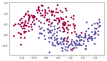
模型以为你实现:
def model(X, Y, layers_dims, optimizer, learning_rate = 0.0007, mini_batch_size = 64, beta = 0.9,
beta1 = 0.9, beta2 = 0.999, epsilon = 1e-8, num_epochs = 10000, print_cost = True):
"""
3-layer neural network model which can be run in different optimizer modes.
Arguments:
X -- input data, of shape (2, number of examples)
Y -- true "label" vector (1 for blue dot / 0 for red dot), of shape (1, number of examples)
layers_dims -- python list, containing the size of each layer
learning_rate -- the learning rate, scalar.
mini_batch_size -- the size of a mini batch
beta -- Momentum hyperparameter
beta1 -- Exponential decay hyperparameter for the past gradients estimates
beta2 -- Exponential decay hyperparameter for the past squared gradients estimates
epsilon -- hyperparameter preventing division by zero in Adam updates
num_epochs -- number of epochs
print_cost -- True to print the cost every 1000 epochs
Returns:
parameters -- python dictionary containing your updated parameters
"""
L = len(layers_dims) # number of layers in the neural networks
costs = [] # to keep track of the cost
t = 0 # initializing the counter required for Adam update
seed = 10 # For grading purposes, so that your "random" minibatches are the same as ours
# Initialize parameters
parameters = initialize_parameters(layers_dims)
# Initialize the optimizer
if optimizer == "gd":
pass # no initialization required for gradient descent
elif optimizer == "momentum":
v = initialize_velocity(parameters)
elif optimizer == "adam":
v, s = initialize_adam(parameters)
# Optimization loop
for i in range(num_epochs):
# Define the random minibatches. We increment the seed to reshuffle differently the dataset after each epoch
seed = seed + 1
minibatches = random_mini_batches(X, Y, mini_batch_size, seed)
for minibatch in minibatches:
# Select a minibatch
(minibatch_X, minibatch_Y) = minibatch
# Forward propagation
a3, caches = forward_propagation(minibatch_X, parameters)
# Compute cost
cost = compute_cost(a3, minibatch_Y)
# Backward propagation
grads = backward_propagation(minibatch_X, minibatch_Y, caches)
# Update parameters
if optimizer == "gd":
parameters = update_parameters_with_gd(parameters, grads, learning_rate)
elif optimizer == "momentum":
parameters, v = update_parameters_with_momentum(parameters, grads, v, beta, learning_rate)
elif optimizer == "adam":
t = t + 1 # Adam counter
parameters, v, s = update_parameters_with_adam(parameters, grads, v, s,
t, learning_rate, beta1, beta2, epsilon)
# Print the cost every 1000 epoch
if print_cost and i % 1000 == 0:
print ("Cost after epoch %i: %f" %(i, cost))
if print_cost and i % 100 == 0:
costs.append(cost)
# plot the cost
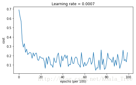
plt.plot(costs)
plt.ylabel('cost')
plt.xlabel('epochs (per 100)')
plt.title("Learning rate = " + str(learning_rate))
plt.show()
return parameters只需调用以下语句观察三个方法的优劣:
train_X, train_Y = load_dataset()
# train 3-layer model
layers_dims = [train_X.shape[0], 5, 2, 1]
#下面三种方法用哪个取消那个注释
#GD方法
#parameters = model(train_X, train_Y, layers_dims, optimizer="gd")
#M方法
#parameters = model(train_X, train_Y, layers_dims, beta=0.9, optimizer="momentum")
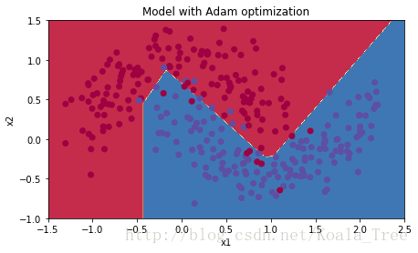
#A方法
#parameters = model(train_X, train_Y, layers_dims, optimizer="adam")
# Predict
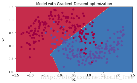
predictions = predict(train_X, train_Y, parameters)
# Plot decision boundary
plt.title("Model with Gradient Descent optimization")
axes = plt.gca()
axes.set_xlim([-1.5, 2.5])
axes.set_ylim([-1, 1.5])
plot_decision_boundary(lambda x: predict_dec(parameters, x.T), train_X, train_Y)小bug:
ng老师的opt_utils.py中的 def initialize_parameters(layer_dims) 里
    for l in range(1, L):
        parameters['W' + str(l)] = np.random.randn(layer_dims[l], layer_dims[l-1])*  np.sqrt(2. / layer_dims[l-1])#ng这里刚开始是2,结果所有W都是0,,,acc=0.5
        parameters['b' + str(l)] = np.zeros((layer_dims[l], 1))

        assert(parameters['W' + str(l)].shape == layer_dims[l], layer_dims[l-1])
        assert(parameters['W' + str(l)].shape == layer_dims[l], 1)
第二行原来是2,结果三种方法的精确度都是0.5且所有权重W值都是0,改成2.就行,同时如果换成1.结果会更好
结果:
MGD:
Cost after epoch 0: 0.690736
Cost after epoch 1000: 0.685273
Cost after epoch 2000: 0.647072
Cost after epoch 3000: 0.619525
Cost after epoch 4000: 0.576584
Cost after epoch 5000: 0.607243
Cost after epoch 6000: 0.529403
Cost after epoch 7000: 0.460768
Cost after epoch 8000: 0.465586
Cost after epoch 9000: 0.464518

Accuracy: 0.796666666667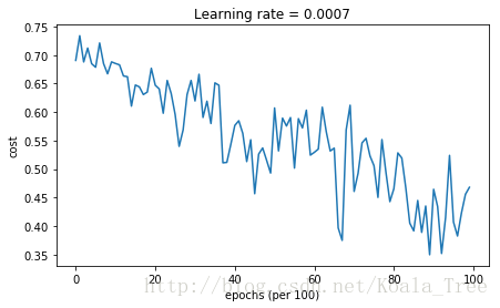
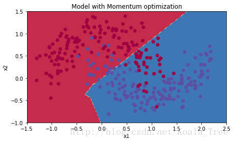
M:
Cost after epoch 0: 0.690741
Cost after epoch 1000: 0.685341
Cost after epoch 2000: 0.647145
Cost after epoch 3000: 0.619594
Cost after epoch 4000: 0.576665
Cost after epoch 5000: 0.607324
Cost after epoch 6000: 0.529476
Cost after epoch 7000: 0.460936
Cost after epoch 8000: 0.465780
Cost after epoch 9000: 0.464740

Accuracy: 0.796666666667
A:
Cost after epoch 0: 0.690552
Cost after epoch 1000: 0.233787
Cost after epoch 2000: 0.179942
Cost after epoch 3000: 0.099978
Cost after epoch 4000: 0.142203
Cost after epoch 5000: 0.114152
Cost after epoch 6000: 0.128446
Cost after epoch 7000: 0.042047
Cost after epoch 8000: 0.132215
Cost after epoch 9000: 0.214512

Accuracy: 0.936666666667
6-总结
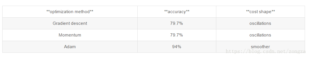
动量通常是有帮助的,但是考虑到学习速度小和数据集过于简单,它的影响几乎是可以忽略的。此外,你在下降过程中看到的巨大振荡来自于这样一个事实,一些小批量数据的优化更难。
另一方面,Adam明显优于小批量梯度下降和动量。如果您在这个简单的数据集上运行这个模型,那么这三种方法都会得到非常好的结果。然而,你已经看到A收敛得更快了。
- Adam paper: https://arxiv.org/pdf/1412.6980.pdf