Initialization
Welcome to the first assignment of “Improving Deep Neural Networks”.
Training your neural network requires specifying an initial value of the weights. A well chosen initialization method will help learning.
If you completed the previous course of this specialization, you probably followed our instructions for weight initialization, and it has worked out so far. But how do you choose the initialization for a new neural network? In this notebook, you will see how different initializations lead to different results.
A well chosen initialization can:
- Speed up the convergence of gradient descent
- Increase the odds of gradient descent converging to a lower training (and generalization) error
To get started, run the following cell to load the packages and the planar dataset you will try to classify.
import numpy as np
import matplotlib.pyplot as plt
import sklearn
import sklearn.datasets
from init_utils import sigmoid, relu, compute_loss, forward_propagation, backward_propagation
from init_utils import update_parameters, predict, load_dataset, plot_decision_boundary, predict_dec


#%matplotlib inline
#其作用就是在你调用plot()进行画图或者直接输入Figure的实例对象的时候,会自动的显示并把figure嵌入到console中。
#魔术命令,可以在notebook中显示用matplotlib绘制的图片。
#其实在新版的jupyter notebook里,有没有这行代码已经没什么差别了

#matplotlib.pyplot.rc     https://translate.google.com/translate?hl=zh-CN&sl=en&u=https://matplotlib.org/&prev=search
#设置当前的rc参数
plt.rcParams['figure.figsize'] = (7.0, 4.0) # set default size of plots
plt.rcParams['image.interpolation'] = 'nearest'
plt.rcParams['image.cmap'] = 'gray'

# load image dataset: blue/red dots in circles
#load_dateset().包含了画图部分
train_X, train_Y, test_X, test_Y = load_dataset()

#print("train_X:",str(train_X.shape))#老规矩,X表位置。Y表0/1。共300个训练集
#print("train_Y:",str(train_Y.shape))
#print("train_Y:",str(test_Y.shape[1])) #100个测试集
You would like a classifier to separate the blue dots from the red dots.
1 - Neural Network model
You will use a 3-layer neural network (already implemented for you). Here are the initialization methods you will experiment with:
- Zeros initialization – setting
initialization = "zeros"in the input argument. - Random initialization – setting
initialization = "random"in the input argument. This initializes the weights to large random values. - He initialization – setting
initialization = "he"in the input argument. This initializes the weights to random values scaled according to a paper by He et al., 2015.
Instructions: Please quickly read over the code below, and run it. In the next part you will implement the three initialization methods that this model() calls.
def model(X, Y, learning_rate = 0.01, num_iterations = 15000, print_cost = True, initialization = "he"):
    """
    Implements a three-layer neural network: LINEAR->RELU->LINEAR->RELU->LINEAR->SIGMOID.

    Arguments:
    X -- input data, of shape (2, number of examples)
    Y -- true "label" vector (containing 0 for red dots; 1 for blue dots), of shape (1, number of examples)
    learning_rate -- learning rate for gradient descent
    num_iterations -- number of iterations to run gradient descent
    print_cost -- if True, print the cost every 1000 iterations
    initialization -- flag to choose which initialization to use ("zeros","random" or "he")

    Returns:
    parameters -- parameters learnt by the model
    """

    grads = {}
    costs = [] # to keep track of the loss
    m = X.shape[1] # number of examples
    layers_dims = [X.shape[0], 10, 5, 1]  #注意这里的第一层。

    # Initialize parameters dictionary.
    if initialization == "zeros":
        parameters = initialize_parameters_zeros(layers_dims)
    elif initialization == "random":
        parameters = initialize_parameters_random(layers_dims)
    elif initialization == "he":
        parameters = initialize_parameters_he(layers_dims)

    # Loop (gradient descent)

    for i in range(0, num_iterations):

        # Forward propagation: LINEAR -> RELU -> LINEAR -> RELU -> LINEAR -> SIGMOID.
        a3, cache = forward_propagation(X, parameters)

        # Loss
        cost = compute_loss(a3, Y)

        # Backward propagation.
        grads = backward_propagation(X, Y, cache)

        # Update parameters.
        parameters = update_parameters(parameters, grads, learning_rate)

        # Print the loss every 1000 iterations
        if print_cost and i % 1000 == 0:
            print("Cost after iteration {}: {}".format(i, cost))
            costs.append(cost)

    # plot the loss
    plt.plot(costs)
    plt.ylabel('cost')
    plt.xlabel('iterations (per hundreds)')
    plt.title("Learning rate =" + str(learning_rate))
    plt.show()

    return parameters
2 - Zero initialization
There are two types of parameters to initialize in a neural network:
- the weight matrices
- the bias vectors
Exercise: Implement the following function to initialize all parameters to zeros. You’ll see later that this does not work well since it fails to “break symmetry”, but lets try it anyway and see what happens. Use np.zeros((…,…)) with the correct shapes.
# GRADED FUNCTION: initialize_parameters_zeros

def initialize_parameters_zeros(layers_dims):
    """
    Arguments:
    layer_dims -- python array (list) containing the size of each layer.

    Returns:
    parameters -- python dictionary containing your parameters "W1", "b1", ..., "WL", "bL":
                    W1 -- weight matrix of shape (layers_dims[1], layers_dims[0])
                    b1 -- bias vector of shape (layers_dims[1], 1)
                    ...
                    WL -- weight matrix of shape (layers_dims[L], layers_dims[L-1])
                    bL -- bias vector of shape (layers_dims[L], 1)
    """

    parameters = {}
    L = len(layers_dims)            # number of layers in the network

    for l in range(1, L):   #layers_dims,是数组,下表最多到L-1
        ### START CODE HERE ### (≈ 2 lines of code)
        parameters['W' + str(l)] = np.zeros((layers_dims[l],layers_dims[l-1]))#注意内层还有括号,这仅是第一个参数
        parameters['b' + str(l)] = np.zeros((layers_dims[l],1))
        ### END CODE HERE ###
    return parameters
parameters = initialize_parameters_zeros([3,2,1])
print("W1 = " + str(parameters["W1"]))
print("b1 = " + str(parameters["b1"]))
print("W2 = " + str(parameters["W2"]))
print("b2 = " + str(parameters["b2"]))
W1 = [[0. 0. 0.]
 [0. 0. 0.]]
b1 = [[0.]
 [0.]]
W2 = [[0. 0.]]
b2 = [[0.]]
Expected Output:
| **W1** | [[ 0. 0. 0.] [ 0. 0. 0.]] |
| **b1** | [[ 0.] [ 0.]] |
| **W2** | [[ 0. 0.]] |
| **b2** | [[ 0.]] |
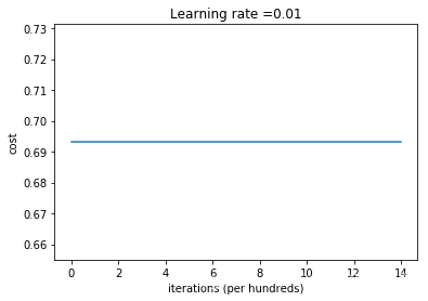
Run the following code to train your model on 15,000 iterations using zeros initialization.
parameters = model(train_X, train_Y, initialization = "zeros")
print ("On the train set:")
predictions_train = predict(train_X, train_Y, parameters)
print ("On the test set:")
predictions_test = predict(test_X, test_Y, parameters)
Cost after iteration 0: 0.6931471805599453
Cost after iteration 1000: 0.6931471805599453
Cost after iteration 2000: 0.6931471805599453
Cost after iteration 3000: 0.6931471805599453
Cost after iteration 4000: 0.6931471805599453
Cost after iteration 5000: 0.6931471805599453
Cost after iteration 6000: 0.6931471805599453
Cost after iteration 7000: 0.6931471805599453
Cost after iteration 8000: 0.6931471805599453
Cost after iteration 9000: 0.6931471805599453
Cost after iteration 10000: 0.6931471805599455
Cost after iteration 11000: 0.6931471805599453
Cost after iteration 12000: 0.6931471805599453
Cost after iteration 13000: 0.6931471805599453
Cost after iteration 14000: 0.6931471805599453
On the train set:
Accuracy: 0.5
On the test set:
Accuracy: 0.5
The performance is really bad, and the cost does not really decrease, and the algorithm performs no better than random guessing. Why? Lets look at the details of the predictions and the decision boundary:
我理解不透彻这里,“本来我们希望不同的结点学习到不同的参数,但是由于参数相同以及输出值都一样,不同的结点根本无法学到不同的特征!这样就失去了网络学习特征的意义了。”???
参考文章:https://zhuanlan.zhihu.com/p/27190255
print ("predictions_train = " + str(predictions_train))
print ("predictions_test = " + str(predictions_test))
predictions_train = [[0 0 0 0 0 0 0 0 0 0 0 0 0 0 0 0 0 0 0 0 0 0 0 0 0 0 0 0 0 0 0 0 0 0 0 0
  0 0 0 0 0 0 0 0 0 0 0 0 0 0 0 0 0 0 0 0 0 0 0 0 0 0 0 0 0 0 0 0 0 0 0 0
  0 0 0 0 0 0 0 0 0 0 0 0 0 0 0 0 0 0 0 0 0 0 0 0 0 0 0 0 0 0 0 0 0 0 0 0
  0 0 0 0 0 0 0 0 0 0 0 0 0 0 0 0 0 0 0 0 0 0 0 0 0 0 0 0 0 0 0 0 0 0 0 0
  0 0 0 0 0 0 0 0 0 0 0 0 0 0 0 0 0 0 0 0 0 0 0 0 0 0 0 0 0 0 0 0 0 0 0 0
  0 0 0 0 0 0 0 0 0 0 0 0 0 0 0 0 0 0 0 0 0 0 0 0 0 0 0 0 0 0 0 0 0 0 0 0
  0 0 0 0 0 0 0 0 0 0 0 0 0 0 0 0 0 0 0 0 0 0 0 0 0 0 0 0 0 0 0 0 0 0 0 0
  0 0 0 0 0 0 0 0 0 0 0 0 0 0 0 0 0 0 0 0 0 0 0 0 0 0 0 0 0 0 0 0 0 0 0 0
  0 0 0 0 0 0 0 0 0 0 0 0]]
predictions_test = [[0 0 0 0 0 0 0 0 0 0 0 0 0 0 0 0 0 0 0 0 0 0 0 0 0 0 0 0 0 0 0 0 0 0 0 0
  0 0 0 0 0 0 0 0 0 0 0 0 0 0 0 0 0 0 0 0 0 0 0 0 0 0 0 0 0 0 0 0 0 0 0 0
  0 0 0 0 0 0 0 0 0 0 0 0 0 0 0 0 0 0 0 0 0 0 0 0 0 0 0 0]]
#plt.title("Model with Zeros initialization")axes = plt.gca()
#axes.set_xlim([-1.5,1.5])
#axes.set_ylim([-1.5,1.5])
#plot_decision_boundary(lambda x: predict_dec(parameters, x.T), train_X, train_Y)
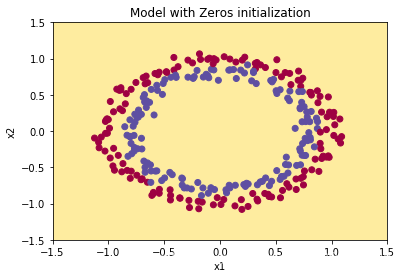
plt.title("Model with Zeros initialization")
axes = plt.gca()
axes.set_xlim([-1.5, 1.5])
axes.set_ylim([-1.5, 1.5])
#plot_decision_boundary(lambda x: predict_dec(parameters, x.T), train_X, train_Y)
plot_decision_boundary(lambda x:predict_dec(parameters, x.T), train_X, train_Y)
#plt.scatter
#需要一个一个二维数组,其中行是RGB或RGBA。
#(400,)是秩为1的数组
#print("train_X.shape:" + str(train_X.shape))
#print("train_X[0].shape:" + str(train_X[0].shape))
#print("train_Y.shape:" + str(train_Y.shape))
train_X.shape:(2, 300)
train_X[0].shape:(300,)
train_Y.shape:(1, 300)
上面的最后一行代码,总是报错
我特地回去查看原函数,但是有些地方不明白。
plot_decision_boundary(model,X,y)。
lambda:是创建隐藏函数
这样,lambda x:predict_dec(parameters, x.T)作为第一个参数传入plot_decision_boundary函数中。
但是,plot_decision_boundary函数中使用该参数的方式是model(np.c_[xx.ravel(), yy.ravel()])。即,将一个链接而成的二维数组作为一维数组的参数。
不怎么明白。
同时,init_utils.py的源文件有需要修改的地方:吴恩达Deeplearning第二课代码bug修正大全
4.修改plt.scatter(X[0, :], X[1, :], c=y, cmap=plt.cm.Spectral)
为plt.scatter(X[0, :], X[1, :], c=y.reshape(X[0,:].shape), cmap=plt.cm.Spectral)
The model is predicting 0 for every example.
In general, initializing all the weights to zero results in the network failing to break symmetry. This means that every neuron in each layer will learn the same thing, and you might as well be training a neural network with for every layer, and the network is no more powerful than a linear classifier such as logistic regression.
**What you should remember**: - The weights $W^{[l]}$ should be initialized randomly to break symmetry. - It is however okay to initialize the biases $b^{[l]}$ to zeros. Symmetry is still broken so long as $W^{[l]}$ is initialized randomly.3 - Random initialization
To break symmetry, lets intialize the weights randomly. Following random initialization, each neuron can then proceed to learn a different function of its inputs. In this exercise, you will see what happens if the weights are intialized randomly, but to very large values.
Exercise: Implement the following function to initialize your weights to large random values (scaled by *10) and your biases to zeros. Use np.random.randn(..,..) * 10 for weights and np.zeros((.., ..)) for biases. We are using a fixed np.random.seed(..) to make sure your “random” weights match ours, so don’t worry if running several times your code gives you always the same initial values for the parameters.
np.random.rand():生成给定形状的随机值
np.random.randn():这个随机值的生成,服从正太分布
# GRADED FUNCTION: initialize_parameters_random

def initialize_parameters_random(layers_dims):
    """
    Arguments:
    layer_dims -- python array (list) containing the size of each layer.

    Returns:
    parameters -- python dictionary containing your parameters "W1", "b1", ..., "WL", "bL":
                    W1 -- weight matrix of shape (layers_dims[1], layers_dims[0])
                    b1 -- bias vector of shape (layers_dims[1], 1)
                    ...
                    WL -- weight matrix of shape (layers_dims[L], layers_dims[L-1])
                    bL -- bias vector of shape (layers_dims[L], 1)
    """

    np.random.seed(3)               # This seed makes sure your "random" numbers will be the as ours
    parameters = {}
    L = len(layers_dims)            # integer representing the number of layers

    for l in range(1, L):
        ### START CODE HERE ### (≈ 2 lines of code)
        ###设置比较大的参数
        parameters['W' + str(l)] = np.random.randn(layers_dims[l],layers_dims[l-1])*10
        parameters['b' + str(l)] = np.zeros((layers_dims[l],1))
        ### END CODE HERE ###

    return parameters
parameters = initialize_parameters_random([3, 2, 1])
print("W1 = " + str(parameters["W1"]))
print("b1 = " + str(parameters["b1"]))
print("W2 = " + str(parameters["W2"]))
print("b2 = " + str(parameters["b2"]))
W1 = [[ 17.88628473   4.36509851   0.96497468]
 [-18.63492703  -2.77388203  -3.54758979]]
b1 = [[0.]
 [0.]]
W2 = [[-0.82741481 -6.27000677]]
b2 = [[0.]]
Expected Output:
| **W1** | [[ 17.88628473 4.36509851 0.96497468] [-18.63492703 -2.77388203 -3.54758979]] |
| **b1** | [[ 0.] [ 0.]] |
| **W2** | [[-0.82741481 -6.27000677]] |
| **b2** | [[ 0.]] |
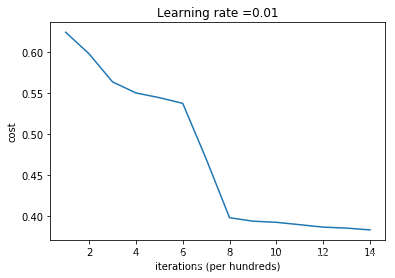
Run the following code to train your model on 15,000 iterations using random initialization.
parameters = model(train_X, train_Y, initialization = "random")
print ("On the train set:")
predictions_train = predict(train_X, train_Y, parameters)
print ("On the test set:")
predictions_test = predict(test_X, test_Y, parameters)
/home/dacao/exercise/Jupyter/deep_learning02/week5/Initialization/init_utils.py:145: RuntimeWarning: divide by zero encountered in log
  logprobs = np.multiply(-np.log(a3),Y) + np.multiply(-np.log(1 - a3), 1 - Y)
/home/dacao/exercise/Jupyter/deep_learning02/week5/Initialization/init_utils.py:145: RuntimeWarning: invalid value encountered in multiply
  logprobs = np.multiply(-np.log(a3),Y) + np.multiply(-np.log(1 - a3), 1 - Y)


Cost after iteration 0: inf
Cost after iteration 1000: 0.6242434241539614
Cost after iteration 2000: 0.5978811277755388
Cost after iteration 3000: 0.5636242569764779
Cost after iteration 4000: 0.5500958254523324
Cost after iteration 5000: 0.544339206192789
Cost after iteration 6000: 0.5373584514307651
Cost after iteration 7000: 0.469574666760224
Cost after iteration 8000: 0.39766324943219844
Cost after iteration 9000: 0.3934423376823982
Cost after iteration 10000: 0.3920158992175907
Cost after iteration 11000: 0.38913979237487845
Cost after iteration 12000: 0.3861261344766218
Cost after iteration 13000: 0.3849694511273874
Cost after iteration 14000: 0.3827489017191917
On the train set:
Accuracy: 0.83
On the test set:
Accuracy: 0.86
If you see “inf” as the cost after the iteration 0, this is because of numerical roundoff; a more numerically sophisticated implementation would fix this. But this isn’t worth worrying about for our purposes.
Anyway, it looks like you have broken symmetry, and this gives better results. than before. The model is no longer outputting all 0s.
print (predictions_train)
print (predictions_test)
[[1 0 1 1 0 0 1 1 1 1 1 0 1 0 0 1 0 1 1 0 0 0 1 0 1 1 1 1 1 1 0 1 1 0 0 1
  1 1 1 1 1 1 1 0 1 1 1 1 0 1 0 1 1 1 1 0 0 1 1 1 1 0 1 1 0 1 0 1 1 1 1 0
  0 0 0 0 1 0 1 0 1 1 1 0 0 1 1 1 1 1 1 0 0 1 1 1 0 1 1 0 1 0 1 1 0 1 1 0
  1 0 1 1 0 0 1 0 0 1 1 0 1 1 1 0 1 0 0 1 0 1 1 1 1 1 1 1 0 1 1 0 0 1 1 0
  0 0 1 0 1 0 1 0 1 1 1 0 0 1 1 1 1 0 1 1 0 1 0 1 1 0 1 0 1 1 1 1 0 1 1 1
  1 0 1 0 1 0 1 1 1 1 0 1 1 0 1 1 0 1 1 0 1 0 1 1 1 0 1 1 1 0 1 0 1 0 0 1
  0 1 1 0 1 1 0 1 1 0 1 1 1 0 1 1 1 1 0 1 0 0 1 1 0 1 1 1 0 0 0 1 1 0 1 1
  1 1 0 1 1 0 1 1 1 0 0 1 0 0 0 1 0 0 0 1 1 1 1 0 0 0 0 1 1 1 1 0 0 1 1 1
  1 1 1 1 0 0 0 1 1 1 1 0]]
[[1 1 1 1 0 1 0 1 1 0 1 1 1 0 0 0 0 1 0 1 0 0 1 0 1 0 1 1 1 1 1 0 0 0 0 1
  0 1 1 0 0 1 1 1 1 1 0 1 1 1 0 1 0 1 1 0 1 0 1 0 1 1 1 1 1 1 1 1 1 0 1 0
  1 1 1 1 1 0 1 0 0 1 0 0 0 1 1 0 1 1 0 0 0 1 1 0 1 1 0 0]]
plt.title("Model with large random initialization")
axes = plt.gca()
axes.set_xlim([-1.5,1.5])
axes.set_ylim([-1.5,1.5])
#plot_decision_boundary(lambda x: predict_dec(parameters, x.T), train_X, train_Y)
plot_decision_boundary(lambda x: predict_dec(parameters, x.T), train_X, train_Y)
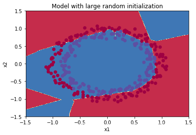
Observations:
- The cost starts very high. This is because with large random-valued weights, the last activation (sigmoid) outputs results that are very close to 0 or 1 for some examples, and when it gets that example wrong it incurs a very high loss for that example. Indeed, when , the loss goes to infinity.
- Poor initialization can lead to vanishing/exploding gradients, which also slows down the optimization algorithm.
- If you train this network longer you will see better results, but initializing with overly large random numbers slows down the optimization.
4 - He initialization
Finally, try “He Initialization”; this is named for the first author of He et al., 2015. (If you have heard of “Xavier initialization”, this is similar except Xavier initialization uses a scaling factor for the weights
of sqrt(1./layers_dims[l-1]) where He initialization would use sqrt(2./layers_dims[l-1]).)
Exercise: Implement the following function to initialize your parameters with He initialization.
Hint: This function is similar to the previous initialize_parameters_random(...). The only difference is that instead of multiplying np.random.randn(..,..) by 10, you will multiply it by
, which is what He initialization recommends for layers with a ReLU activation.
# GRADED FUNCTION: initialize_parameters_he

def initialize_parameters_he(layers_dims):
    """
    Arguments:
    layer_dims -- python array (list) containing the size of each layer.

    Returns:
    parameters -- python dictionary containing your parameters "W1", "b1", ..., "WL", "bL":
                    W1 -- weight matrix of shape (layers_dims[1], layers_dims[0])
                    b1 -- bias vector of shape (layers_dims[1], 1)
                    ...
                    WL -- weight matrix of shape (layers_dims[L], layers_dims[L-1])
                    bL -- bias vector of shape (layers_dims[L], 1)
    """

    np.random.seed(3)
    parameters = {}
    L = len(layers_dims) - 1 # integer representing the number of layers

    for l in range(1, L + 1):
        ### START CODE HERE ### (≈ 2 lines of code)
        ####初始化参数,不能过大。用乘以前一层维数分之一的2被,开根号
        parameters['W' + str(l)] = np.random.randn(layers_dims[l], layers_dims[l - 1]) * np.sqrt(2 / layers_dims[l - 1])
        parameters['b' + str(l)] = np.zeros((layers_dims[l],1))
        ### END CODE HERE ###

    return parameters
parameters = initialize_parameters_he([2, 4, 1])
print("W1 = " + str(parameters["W1"]))
print("b1 = " + str(parameters["b1"]))
print("W2 = " + str(parameters["W2"]))
print("b2 = " + str(parameters["b2"]))
W1 = [[ 1.78862847  0.43650985]
 [ 0.09649747 -1.8634927 ]
 [-0.2773882  -0.35475898]
 [-0.08274148 -0.62700068]]
b1 = [[0.]
 [0.]
 [0.]
 [0.]]
W2 = [[-0.03098412 -0.33744411 -0.92904268  0.62552248]]
b2 = [[0.]]
Expected Output:
| **W1** | [[ 1.78862847 0.43650985] [ 0.09649747 -1.8634927 ] [-0.2773882 -0.35475898] [-0.08274148 -0.62700068]] |
| **b1** | [[ 0.] [ 0.] [ 0.] [ 0.]] |
| **W2** | [[-0.03098412 -0.33744411 -0.92904268 0.62552248]] |
| **b2** | [[ 0.]] |
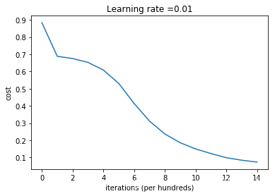
Run the following code to train your model on 15,000 iterations using He initialization.
parameters = model(train_X, train_Y, initialization = "he")
print ("On the train set:")
predictions_train = predict(train_X, train_Y, parameters)
print ("On the test set:")
predictions_test = predict(test_X, test_Y, parameters)
Cost after iteration 0: 0.8830537463419761
Cost after iteration 1000: 0.6879825919728063
Cost after iteration 2000: 0.6751286264523371
Cost after iteration 3000: 0.6526117768893807
Cost after iteration 4000: 0.6082958970572938
Cost after iteration 5000: 0.5304944491717495
Cost after iteration 6000: 0.4138645817071794
Cost after iteration 7000: 0.3117803464844441
Cost after iteration 8000: 0.23696215330322562
Cost after iteration 9000: 0.18597287209206834
Cost after iteration 10000: 0.15015556280371806
Cost after iteration 11000: 0.12325079292273546
Cost after iteration 12000: 0.09917746546525934
Cost after iteration 13000: 0.08457055954024278
Cost after iteration 14000: 0.07357895962677369
On the train set:
Accuracy: 0.9933333333333333
On the test set:
Accuracy: 0.96
plt.title("Model with He initialization")
axes = plt.gca()
axes.set_xlim([-1.5,1.5])
axes.set_ylim([-1.5,1.5])
plot_decision_boundary(lambda x: predict_dec(parameters, x.T), train_X, train_Y)
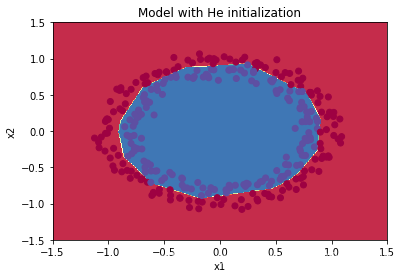
Observations:
- The model with He initialization separates the blue and the red dots very well in a small number of iterations.
5 - Conclusions
You have seen three different types of initializations. For the same number of iterations and same hyperparameters the comparison is:
</tr>
    <td>
    3-layer NN with zeros initialization
    </td>
    <td>
    50%
    </td>
    <td>
    fails to break symmetry
    </td>
<tr>
    <td>
    3-layer NN with large random initialization
    </td>
    <td>
    83%
    </td>
    <td>
    too large weights
    </td>
</tr>
<tr>
    <td>
    3-layer NN with He initialization
    </td>
    <td>
    99%
    </td>
    <td>
    recommended method
    </td>
</tr>
| **Model** | **Train accuracy** | **Problem/Comment** |