题目太长啦!文档下载【传送门】
第1题
简述:实现逻辑回归。
此处使用了minimize函数代替Matlab的fminunc函数,参考了该博客【传送门】。
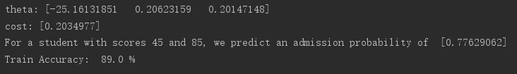
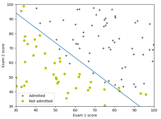
 1 import numpy as np
 2 import matplotlib.pyplot as plt
 3 import scipy.optimize as op
 4
 5 #S函数
 6 def sigmoid(z):
 7     g = 1/(1+np.exp(-z))
 8     return g
 9
10 #cost计算函数
11 def costFunction(theta, X, y):
12     theta = np.array(theta).reshape((np.size(theta),1))
13     m = np.size(y)
14     h = sigmoid(np.dot(X, theta))
15     J = 1/m*(-np.dot(y.T, np.log(h)) - np.dot((1-y.T), np.log(1-h)))
16     return J.flatten()
17
18 def gradient(theta, X, y):
19     theta = np.array(theta).reshape((np.size(theta), 1))
20     m = np.size(y)
21     h = sigmoid(np.dot(X, theta))
22     grad = 1/m*np.dot(X.T, h - y)
23     return grad.flatten()
24
25
26 #读取数据,第一列是成绩1,第二列是成绩2,第三列是yes/no
27 data = np.loadtxt('ex2data1.txt', delimiter=',', dtype='float')
28 m = np.size(data[:, 0])
29 # print(data)
30
31 #绘制样本点
32 X = data[:, 0:2]
33 y = data[:, 2:3]
34 pos = np.where(y == 1)[0]
35 neg = np.where(y == 0)[0]
36 X1 = X[pos, 0:2]
37 X0 = X[neg, 0:2]
38 plt.plot(X1[:, 0], X1[:, 1], 'k+')
39 plt.plot(X0[:, 0], X0[:, 1], 'yo')
40 plt.xlabel('Exam 1 score')
41 plt.ylabel('Exam 2 score')
42
43 #求解最优解
44 one = np.ones(m)
45 X = np.insert(X, 0, values=one, axis=1)
46 initial_theta = np.zeros(np.size(X, 1))
47 result = op.minimize(fun=costFunction, x0=initial_theta, args=(X, y), method='TNC', jac=gradient)
48 # print(result)
49 theta = result.x
50 cost = result.fun
51 print('theta:', theta)
52 print('cost:', cost)
53
54 #绘制决策边界
55 plot_x = np.array([np.min(X[:, 1]), np.max(X[:, 2])])
56 # print(plot_x)
57 plot_y = (-1/theta[2])*(theta[1]*plot_x+theta[0])
58 # print(plot_y)
59 plt.plot(plot_x,plot_y)
60 plt.legend(labels=['Admitted', 'Not admitted'])
61 plt.axis([30, 100, 30, 100])
62 plt.show()
63
64 #预测[45 85]成绩的学生,并计算准确率
65 theta = np.array(theta).reshape((np.size(theta),1))
66 z = np.dot([1, 45, 85], theta)
67 prob = sigmoid(z)
68 print('For a student with scores 45 and 85, we predict an admission probability of ', prob)
69 p = np.round(sigmoid(np.dot(X,theta)))
70 acc = np.mean(p==y)*100
71 print('Train Accuracy: ',acc,'%')
运行结果:
第2题
简述:通过正规化实现逻辑回归。
 1 import numpy as np
 2 import matplotlib.pyplot as plt
 3 import scipy.optimize as op
 4
 5 #S函数
 6 def sigmoid(z):
 7     g = 1/(1+np.exp(-z))
 8     return g
 9
10 #cost计算函数
11 def costFunction(theta, X, y, lamb):
12     theta = np.array(theta).reshape((np.size(theta), 1))
13     m = np.size(y)
14     h = sigmoid(np.dot(X, theta))
15     J = 1/m*(-np.dot(y.T, np.log(h)) - np.dot((1-y.T), np.log(1-h)))
16     # 添加项
17     theta2 = theta[1:, 0]
18     Jadd = lamb/(2*m)*np.sum(theta2**2)
19     J = J + Jadd
20     return J.flatten()
21
22 #求梯度
23 def gradient(theta, X, y, lamb):
24     theta = np.array(theta).reshape((np.size(theta), 1))
25     m = np.size(y)
26     h = sigmoid(np.dot(X, theta))
27     grad = 1/m*np.dot(X.T, h - y)
28     #添加项
29     theta[0,0] = 0
30     gradadd = lamb/m*theta
31     grad = grad + gradadd
32     return grad.flatten()
33
34 #求特征矩阵
35 def mapFeature(X1, X2):
36     degree = 6
37     out = np.ones((np.size(X1),1))
38     for i in range(1, degree+1):
39         for j in range(0, i+1):
40             res = np.multiply(np.power(X1, i-j), np.power(X2, j))
41             out = np.insert(out, np.size(out[0, :]), values=res, axis=1)
42     return out
43
44
45
46 #读取数据,第一列是成绩1,第二列是成绩2,第三列是yes/no
47 data = np.loadtxt('ex2data2.txt', delimiter=',', dtype='float')
48 m = np.size(data[:, 0])
49
50 #绘制样本点
51 X = data[:, 0:2]
52 y = data[:, 2:3]
53 pos = np.where(y == 1)[0]
54 neg = np.where(y == 0)[0]
55 X1 = X[pos, 0:2]
56 X0 = X[neg, 0:2]
57 plt.plot(X1[:, 0], X1[:, 1], 'k+')
58 plt.plot(X0[:, 0], X0[:, 1], 'yo')
59 plt.xlabel('Microchip Test 1')
60 plt.ylabel('Microchip Test 2')
61 plt.legend(labels=['y = 1', 'y = 0'])
62
63 #数据初始化
64 X = mapFeature(X[:, 0], X[:, 1])
65 # print(X)
66 lamb = 1
67 initial_theta = np.zeros(np.size(X, 1))
68
69 #求解最优解
70 result = op.minimize(fun=costFunction, x0=initial_theta, args=(X, y, lamb), method='TNC', jac=gradient)
71 # print(result)
72 cost = result.fun
73 theta = result.x
74 print('theta:', theta)
75 print('cost:', cost)
76
77 #绘制决策边界
78 u = np.linspace(-1, 1.5, 50)
79 v = np.linspace(-1, 1.5, 50)
80 z = np.zeros((np.size(u),np.size(v)))
81 theta = np.array(theta).reshape((np.size(theta), 1))
82 for i in range(0, np.size(u)):
83     for j in range(0, np.size(v)):
84         z[i, j] = np.dot(mapFeature(u[i], v[j]), theta)
85 # print(z)
86 plt.contour(u, v, z.T, [0])
87 plt.show()
88
89 #计算准确率
90 p = np.round(sigmoid(np.dot(X,theta)))
91 acc = np.mean(p==y)*100
92 print('Train Accuracy: ',acc,'%')
运行结果:

