【吴恩达】机器学习作业ex2data1--逻辑回归（python）

1.前言

        看到了逻辑回归，今天就把逻辑回归也写了一下，问题是预测一个学生是否被大学录取，有一些历史数据，要根据这些历史数据来建立逻辑回归。

2.数据

简述：第一列是学生的成绩1，第二列是学生的成绩2，第三列是录取结果（0-失败/1-成功）

使用方法：新建一个txt的文本，将这些数据原封不动的复制进去就可以

34.62365962451697,78.0246928153624,0
30.28671076822607,43.89499752400101,0
35.84740876993872,72.90219802708364,0
60.18259938620976,86.30855209546826,1
79.0327360507101,75.3443764369103,1
45.08327747668339,56.3163717815305,0
61.10666453684766,96.51142588489624,1
75.02474556738889,46.55401354116538,1
76.09878670226257,87.42056971926803,1
84.43281996120035,43.53339331072109,1
95.86155507093572,38.22527805795094,0
75.01365838958247,30.60326323428011,0
82.30705337399482,76.48196330235604,1
69.36458875970939,97.71869196188608,1
39.53833914367223,76.03681085115882,0
53.9710521485623,89.20735013750205,1
69.07014406283025,52.74046973016765,1
67.94685547711617,46.67857410673128,0
70.66150955499435,92.92713789364831,1
76.97878372747498,47.57596364975532,1
67.37202754570876,42.83843832029179,0
89.67677575072079,65.79936592745237,1
50.534788289883,48.85581152764205,0
34.21206097786789,44.20952859866288,0
77.9240914545704,68.9723599933059,1
62.27101367004632,69.95445795447587,1
80.1901807509566,44.82162893218353,1
93.114388797442,38.80067033713209,0
61.83020602312595,50.25610789244621,0
38.78580379679423,64.99568095539578,0
61.379289447425,72.80788731317097,1
85.40451939411645,57.05198397627122,1
52.10797973193984,63.12762376881715,0
52.04540476831827,69.43286012045222,1
40.23689373545111,71.16774802184875,0
54.63510555424817,52.21388588061123,0
33.91550010906887,98.86943574220611,0
64.17698887494485,80.90806058670817,1
74.78925295941542,41.57341522824434,0
34.1836400264419,75.2377203360134,0
83.90239366249155,56.30804621605327,1
51.54772026906181,46.85629026349976,0
94.44336776917852,65.56892160559052,1
82.36875375713919,40.61825515970618,0
51.04775177128865,45.82270145776001,0
62.22267576120188,52.06099194836679,0
77.19303492601364,70.45820000180959,1
97.77159928000232,86.7278223300282,1
62.07306379667647,96.76882412413983,1
91.56497449807442,88.69629254546599,1
79.94481794066932,74.16311935043758,1
99.2725269292572,60.99903099844988,1
90.54671411399852,43.39060180650027,1
34.52451385320009,60.39634245837173,0
50.2864961189907,49.80453881323059,0
49.58667721632031,59.80895099453265,0
97.64563396007767,68.86157272420604,1
32.57720016809309,95.59854761387875,0
74.24869136721598,69.82457122657193,1
71.79646205863379,78.45356224515052,1
75.3956114656803,85.75993667331619,1
35.28611281526193,47.02051394723416,0
56.25381749711624,39.26147251058019,0
30.05882244669796,49.59297386723685,0
44.66826172480893,66.45008614558913,0
66.56089447242954,41.09209807936973,0
40.45755098375164,97.53518548909936,1
49.07256321908844,51.88321182073966,0
80.27957401466998,92.11606081344084,1
66.74671856944039,60.99139402740988,1
32.72283304060323,43.30717306430063,0
64.0393204150601,78.03168802018232,1
72.34649422579923,96.22759296761404,1
60.45788573918959,73.09499809758037,1
58.84095621726802,75.85844831279042,1
99.82785779692128,72.36925193383885,1
47.26426910848174,88.47586499559782,1
50.45815980285988,75.80985952982456,1
60.45555629271532,42.50840943572217,0
82.22666157785568,42.71987853716458,0
88.9138964166533,69.80378889835472,1
94.83450672430196,45.69430680250754,1
67.31925746917527,66.58935317747915,1
57.23870631569862,59.51428198012956,1
80.36675600171273,90.96014789746954,1
68.46852178591112,85.59430710452014,1
42.0754545384731,78.84478600148043,0
75.47770200533905,90.42453899753964,1
78.63542434898018,96.64742716885644,1
52.34800398794107,60.76950525602592,0
94.09433112516793,77.15910509073893,1
90.44855097096364,87.50879176484702,1
55.48216114069585,35.57070347228866,0
74.49269241843041,84.84513684930135,1
89.84580670720979,45.35828361091658,1
83.48916274498238,48.38028579728175,1
42.2617008099817,87.10385094025457,1
99.31500880510394,68.77540947206617,1
55.34001756003703,64.9319380069486,1
74.77589300092767,89.52981289513276,1

3. 代码块细说

1） 导入经典的三个工具包

import numpy as np
import pandas as pd
import matplotlib.pyplot as plt

2）数据准备

        总体流程就是导出数据，列值命名，插入第一列为后面矩阵乘法做准备，取前三列为x矩阵，最后一列为y矩阵，theta初始化为一个3*1的零矩阵

# 先取出数据
data = pd.read_csv('ex2data1.txt', names=['grade1', 'grade2', 'is_commmitted'])
# 将数据归一化
# data = (data - data.mean()) / data.std()
data.insert(0, 'ones', 1)  # 在头部插入一列1
x = data.iloc[:, 0:3]  # 行全要，x获取前三列
y = data.iloc[:, 3:4]  # 行全要,y获取最后一列
# 将x,y转换为矩阵
x = np.matrix(x)
y = np.matrix(y)
theta = np.matrix(np.zeros((3, 1)))  # 初始化theta为一个3*1维的矩阵

3）预测函数

         我们需要将预测函数的值控制在0-1之间，这样在以后就可以通过0.5作为分界来预估是否被录取，g括号里的内容还是和线性回归一样，进行矩阵相乘，只不过这次我们需要控制值得范围了

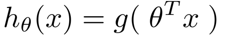
  注意看，这个函数块返回得还是一个矩阵，只不过这里矩阵得内容全部都被控制在了0-1之间 

# 预测的函数h(x)
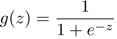
def sigmode(z):
    return 1 / (1 + np.exp(-z))  # np.exp()在这里将矩阵的每一个值都进行了e为底的变化

预测函数的大致图像如下

# 预测函数的大致图像
def hx_pic():
    x = np.arange(-10, 10, 0.01)  # x轴-10到10,间隔0.01
    y = sigmode(x)
    plt.plot(x, y, c='r', linestyle='dashdot', label='$g(Z)$')  # 设置x,y坐标，颜色，画线风格，标签
    plt.xlabel('z')  # x轴标签
    plt.ylabel('hx')  # y轴标签
    plt.legend(loc='best')  # 画线的标签位置
    plt.show()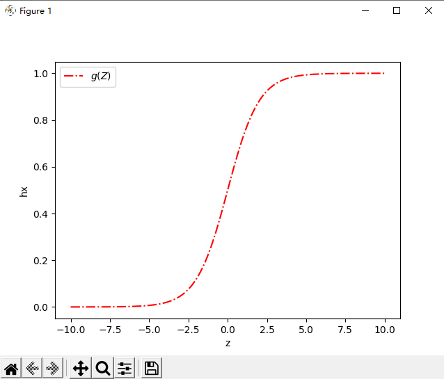

4）代价函数

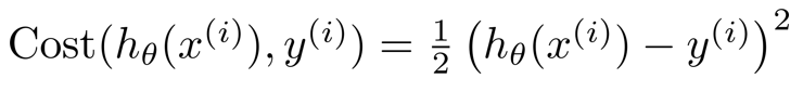
这是以前线性回归的代价函数

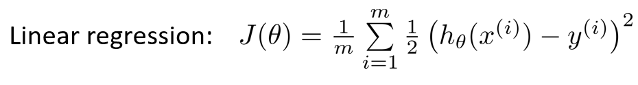
        将后面一部分看作是一个整体，代价函数的主体部分，如果继续用线性回归的代价函数，得到的图像并不是凸函数，可以想象图像必定是一个心电图似的图像，有许多个极小值点，很难准确的找到最小值

         所以我们需要利用下面这个公式来确定代价函数的图像，可以知道log在0-1上是一个单调的函数，同时再将其设为分段函数，就很容易找到最优解

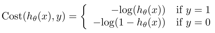
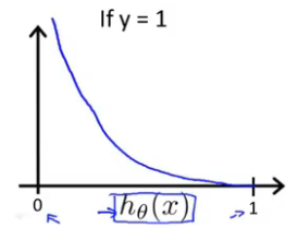
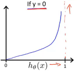
         最后我们再将上述俩个式子合成一个公式，当y = 0 时，前面的一部分会为0，仅执行后面的公式，当y = 1 时，后面的部分会变为0，执行前面的公式

# 代价函数
def cost_fuc(x, y, theta):
    cost_y1 = -(np.log(sigmode(x @ theta)).T @ y)  # 第一部分公式
    cost_y0 = -(np.log(1 - (sigmode(x @ theta))).T @ (1 - y))  #第二部分公式
    return (cost_y1 + cost_y0)/len(x)
    pass

5）梯度下降算法

        梯度下降算法和线性回归中的看着是无差别的，但是要注意，这里的h(x)已经发生了变化，并不是一元的线性方程了，如果不知道theta这里是怎么更新的，可以去看我上一篇文章，里面有theta矩阵在这一步的推导

 

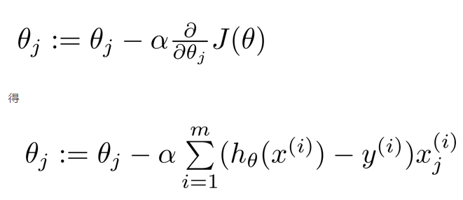
# 梯度下降算法
def gradient_decent(x, y, theta, alpha, update_times):
    cost_list = []
    for i in range(update_times):
        theta = theta - (alpha / len(x)) * (x.T @ (sigmode(x @ theta) - y))
        cost = cost_fuc(x, y, theta)
        cost_list.append(cost)
    return theta, cost_list
    pass

6）预测正确率

         预测正确率的意思其实就是看你得出来的theta准确率能达到多少，因为范围一定是在0-1之间，0.5作为分界条件，用预测准确的个数比上总数即为正确率（我写的会繁琐一些，python的语法还不够精通）

# 预测正确率(实质就是看推测出来的theta值与给定数值的正确率)
def predic_fuc(x, y, theta):
    ct = 0
    t = 0
    p_lst = []
    p_range = sigmode(x @ theta)  # 先将h(x)预测出来的矩阵放入p_range中，里面都是0-1范围的值
    # 循环判断p_range每一行的值，与0.5进行比较，大于等于就默认为被录取，设为1，相反设为0，这些全部存入p_lst列表中
    for i in p_range:
        if i >= 0.5:
            p_lst.append(1)
        elif i < 0.5:
            p_lst.append(0)
    # 将p_lst中预测的值循环与y矩阵中给定的值进行比较，求出相同的次数
    while True:
        if p_lst[t] == y[t]:
            ct += 1
        t += 1
        if t == 100:
            break
    return ct / len(x)  # 返回预测准确的占总数的百分比
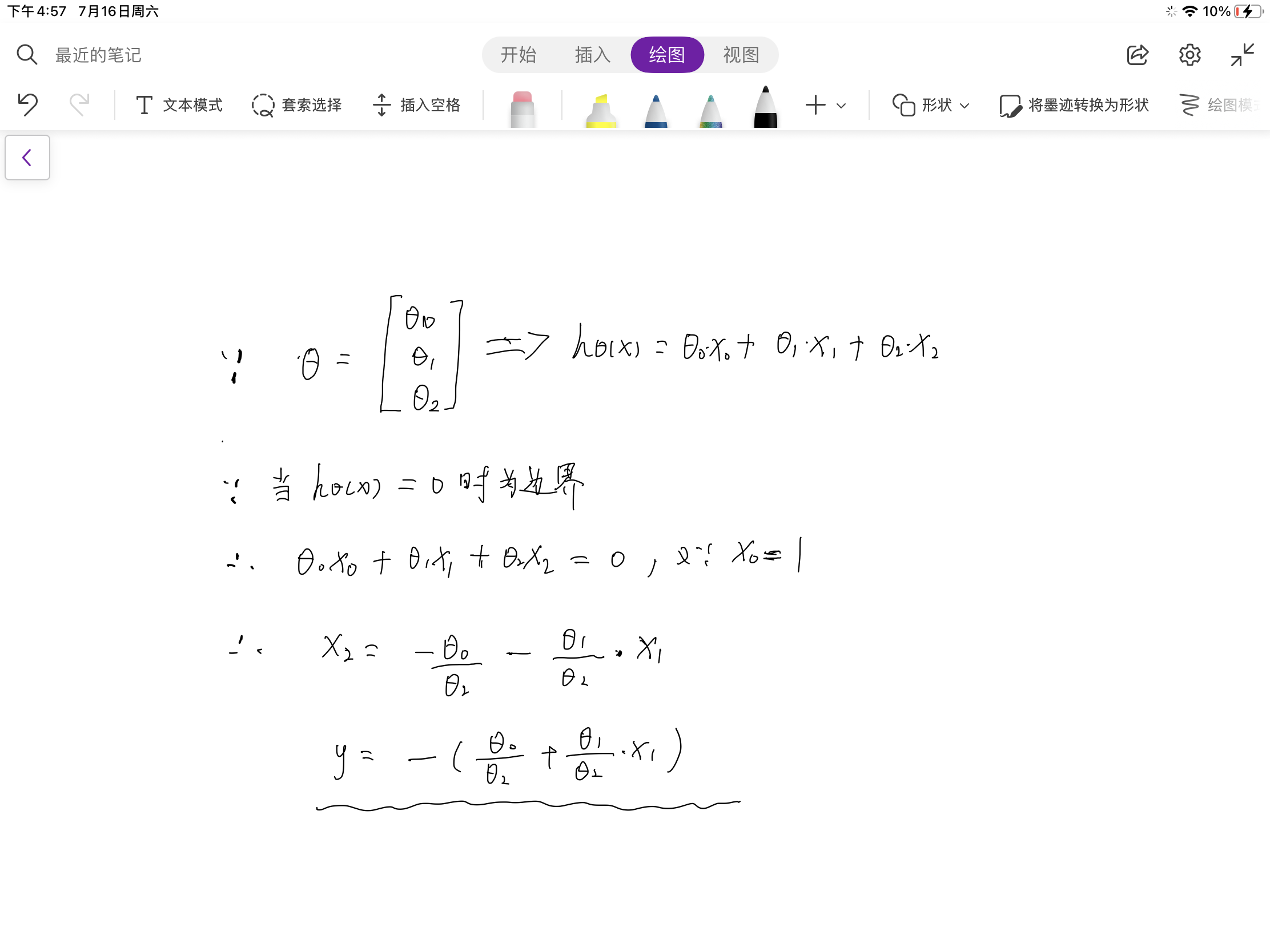
    pass

7）边界图

        这里的theta参数是默认为已经得到了最优解，边界含义其实就是让hθ​(x) = 0，然后导出一个二元一次方程即可，推导过程如下

# 边界图
def boudary_line(theta):
    coef1 = - theta[0, 0] / theta[2, 0]  # 第一个系数
    coef2 = - theta[1, 0] / theta[2, 0]  # 第二个系数
    x = np.arange(0, 130, 0.01)
    f = coef1 + coef2 * x



    positive = data[data['is_commmitted'].isin([1])]  # 找出所有录取结果为1的所有行
    negative = data[data['is_commmitted'].isin([0])]  # 找出所有录取结果为0的所有行
    # 下面是散点图
    fig, ax = plt.subplots(figsize=(12, 8))
    # positive[grade1]就是在所有录取结果为1的行中取出grade1那一列的数据为x轴，并且结果为1的行中grade2为y轴
    ax.scatter(x=positive['grade1'], y=positive['grade2'], s=50, color='purple', marker='o', label='commmitted')
    # positive[grade1]就是在所有录取结果为0的行中取出grade1那一列的数据为x轴，并且结果为0的行中grade2为y轴
    ax.scatter(x=negative['grade1'], y=negative['grade2'], s=50, color='orange', marker='x', label='no_commmitted')
    plt.legend()  # 图例的位置
    ax.set_xlabel('grade1')  # 设置x轴的标题
    ax.set_ylabel('grade1')  # 设置y轴的标题
    plt.plot(x, f, 0.01)  # 部署边界线
    plt.show()
    pass

8）成果展示

theta1, cost_list = gradient_decent(x, y, theta, 0.003, 200000)
print(f'预测成功率为：{predic_fuc(x, y, theta1)}')
boudary_line(theta1)

 边界图

 成功率

 4.全部代码

import numpy as np
import pandas as pd
import matplotlib.pyplot as plt

# 先取出数据
data = pd.read_csv('ex2data1.txt', names=['grade1', 'grade2', 'is_commmitted'])
# 将数据归一化
# data = (data - data.mean()) / data.std()
data.insert(0, 'ones', 1)  # 在头部插入一列1
x = data.iloc[:, 0:3]  # 行全要，x获取前三列
y = data.iloc[:, 3:4]  # 行全要,y获取最后一列
# 将x,y转换为矩阵
x = np.matrix(x)
y = np.matrix(y)
theta = np.matrix(np.zeros((3, 1)))  # 初始化theta为一个3*1维的矩阵


# 预测的函数h(x)
def sigmode(z):
    return 1 / (1 + np.exp(-z))  # np.exp()在这里将矩阵的每一个值都进行了e为底的变化


# 代价函数
def cost_fuc(x, y, theta):
    cost_y1 = -(np.log(sigmode(x @ theta)).T @ y)  # 第一部分公式
    cost_y0 = -(np.log(1 - (sigmode(x @ theta))).T @ (1 - y))  #第二部分公式
    return (cost_y1 + cost_y0)/len(x)
    pass


# print(cost_fuc())  # 看一下初始代价函数

# 梯度下降算法
def gradient_decent(x, y, theta, alpha, update_times):
    cost_list = []
    for i in range(update_times):
        theta = theta - (alpha / len(x)) * (x.T @ (sigmode(x @ theta) - y))
        cost = cost_fuc(x, y, theta)
        cost_list.append(cost)
    return theta, cost_list
    pass


# 边界图
def boudary_line(theta):
    coef1 = - theta[0, 0] / theta[2, 0]  # 第一个系数
    coef2 = - theta[1, 0] / theta[2, 0]  # 第二个系数
    x = np.arange(0, 130, 0.01)
    f = coef1 + coef2 * x


    positive = data[data['is_commmitted'].isin([1])]  # 找出所有录取结果为1的所有行
    negative = data[data['is_commmitted'].isin([0])]  # 找出所有录取结果为0的所有行
    # 下面是散点图
    fig, ax = plt.subplots(figsize=(12, 8))
    # positive[grade1]就是在所有录取结果为1的行中取出grade1那一列的数据为x轴，并且结果为1的行中grade2为y轴
    ax.scatter(x=positive['grade1'], y=positive['grade2'], s=50, color='purple', marker='o', label='committed')
    # positive[grade1]就是在所有录取结果为0的行中取出grade1那一列的数据为x轴，并且结果为0的行中grade2为y轴
    ax.scatter(x=negative['grade1'], y=negative['grade2'], s=50, color='orange', marker='x', label='not_committed')
    plt.legend()  # 图例的位置
    ax.set_xlabel('grade1')  # 设置x轴的标题
    ax.set_ylabel('grade1')  # 设置y轴的标题
    plt.plot(x, f, 0.01)  # 部署边界线
    plt.show()
    pass


# 预测正确率(实质就是看推测出来的theta值与给定数值的正确率)
def predic_fuc(x, y, theta):
    ct = 0
    t = 0
    p_lst = []
    p_range = sigmode(x @ theta)  # 先将h(x)预测出来的矩阵放入p_range中，里面都是0-1范围的值
    # 循环判断p_range每一行的值，与0.5进行比较，大于等于就默认为被录取，设为1，相反设为0，这些全部存入p_lst列表中
    for i in p_range:
        if i >= 0.5:
            p_lst.append(1)
        elif i < 0.5:
            p_lst.append(0)
    # 将p_lst中预测的值循环与y矩阵中给定的值进行比较，求出相同的次数
    while True:
        if p_lst[t] == y[t]:
            ct += 1
        t += 1
        if t == 100:
            break
    return ct / len(x)  # 返回预测准确的占总数的百分比
    pass


# 预测函数的大致图像
def hx_pic():
    x = np.arange(-10, 10, 0.01)  # x轴-10到10,间隔0.01
    y = sigmode(x)
    plt.plot(x, y, c='r', linestyle='dashdot', label='$g(Z)$')  # 设置x,y坐标，颜色，画线风格，标签
    plt.xlabel('z')  # x轴标签
    plt.ylabel('hx')  # y轴标签
    plt.legend(loc='best')  # 画线的标签位置
    plt.show()


theta1, cost_list = gradient_decent(x, y, theta, 0.003, 200000)
print(f'预测成功率为：{predic_fuc(x, y, theta1)}')
boudary_line(theta1)