一.前言
这篇是逻辑回归第一个任务的一个稍改动版,简单说一下代码的流程,需要知道细节的可以看看我前俩篇的逻辑回归,这俩篇分别是单分类和多分类逻辑回归,内容很细,这篇主要是为了上传一下完整代码
二.数据集
0.051267,0.69956,1
-0.092742,0.68494,1
-0.21371,0.69225,1
-0.375,0.50219,1
-0.51325,0.46564,1
-0.52477,0.2098,1
-0.39804,0.034357,1
-0.30588,-0.19225,1
0.016705,-0.40424,1
0.13191,-0.51389,1
0.38537,-0.56506,1
0.52938,-0.5212,1
0.63882,-0.24342,1
0.73675,-0.18494,1
0.54666,0.48757,1
0.322,0.5826,1
0.16647,0.53874,1
-0.046659,0.81652,1
-0.17339,0.69956,1
-0.47869,0.63377,1
-0.60541,0.59722,1
-0.62846,0.33406,1
-0.59389,0.005117,1
-0.42108,-0.27266,1
-0.11578,-0.39693,1
0.20104,-0.60161,1
0.46601,-0.53582,1
0.67339,-0.53582,1
-0.13882,0.54605,1
-0.29435,0.77997,1
-0.26555,0.96272,1
-0.16187,0.8019,1
-0.17339,0.64839,1
-0.28283,0.47295,1
-0.36348,0.31213,1
-0.30012,0.027047,1
-0.23675,-0.21418,1
-0.06394,-0.18494,1
0.062788,-0.16301,1
0.22984,-0.41155,1
0.2932,-0.2288,1
0.48329,-0.18494,1
0.64459,-0.14108,1
0.46025,0.012427,1
0.6273,0.15863,1
0.57546,0.26827,1
0.72523,0.44371,1
0.22408,0.52412,1
0.44297,0.67032,1
0.322,0.69225,1
0.13767,0.57529,1
-0.0063364,0.39985,1
-0.092742,0.55336,1
-0.20795,0.35599,1
-0.20795,0.17325,1
-0.43836,0.21711,1
-0.21947,-0.016813,1
-0.13882,-0.27266,1
0.18376,0.93348,0
0.22408,0.77997,0
0.29896,0.61915,0
0.50634,0.75804,0
0.61578,0.7288,0
0.60426,0.59722,0
0.76555,0.50219,0
0.92684,0.3633,0
0.82316,0.27558,0
0.96141,0.085526,0
0.93836,0.012427,0
0.86348,-0.082602,0
0.89804,-0.20687,0
0.85196,-0.36769,0
0.82892,-0.5212,0
0.79435,-0.55775,0
0.59274,-0.7405,0
0.51786,-0.5943,0
0.46601,-0.41886,0
0.35081,-0.57968,0
0.28744,-0.76974,0
0.085829,-0.75512,0
0.14919,-0.57968,0
-0.13306,-0.4481,0
-0.40956,-0.41155,0
-0.39228,-0.25804,0
-0.74366,-0.25804,0
-0.69758,0.041667,0
-0.75518,0.2902,0
-0.69758,0.68494,0
-0.4038,0.70687,0
-0.38076,0.91886,0
-0.50749,0.90424,0
-0.54781,0.70687,0
0.10311,0.77997,0
0.057028,0.91886,0
-0.10426,0.99196,0
-0.081221,1.1089,0
0.28744,1.087,0
0.39689,0.82383,0
0.63882,0.88962,0
0.82316,0.66301,0
0.67339,0.64108,0
1.0709,0.10015,0
-0.046659,-0.57968,0
-0.23675,-0.63816,0
-0.15035,-0.36769,0
-0.49021,-0.3019,0
-0.46717,-0.13377,0
-0.28859,-0.060673,0
-0.61118,-0.067982,0
-0.66302,-0.21418,0
-0.59965,-0.41886,0
-0.72638,-0.082602,0
-0.83007,0.31213,0
-0.72062,0.53874,0
-0.59389,0.49488,0
-0.48445,0.99927,0
-0.0063364,0.99927,0
0.63265,-0.030612,0
三.代码
1.导入包
import numpy as np
import pandas as pd
import matplotlib.pyplot as plt
2.取出数据
# 先取出数据
data = pd.read_csv('ex2data2.txt', names=['grade1', 'grade2', 'is_commmitted'])
3.设置决策边界函数
设置此函数的目的是建立一个拟合度比较好的决策边界,这里我设置的是普通圆的方程,也可以像其他大神那样写俩个for循环建立更高阶,我这个会相对简单一些,F10就代表x1的1次方和x2的零次方
def feature_mapping(x1, x2):
    data = {}
    data['F10'] = x1
    data['F01'] = x2
    data['F20'] = np.power(x1, 2)
    data['F02'] = np.power(x2, 2)
    data['F11'] = x1 * x2
    return pd.DataFrame(data)
这里补充一下,如果设置的函数阶数过高可能就会出现下面的过拟合的状况,过少又会少拟合,所以大家可以根据不同的状况来选择不同的函数
4.数据初始化
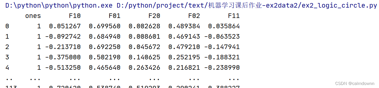
还是先取出俩列特征值x1和x2,将这俩列放入feature_mapping中得到新的函数,并且在第一列加入1,
x1 = data['grade1']
x2 = data['grade2']
data2 = feature_mapping(x1, x2)
data2.insert(0, 'ones', 1)
x_new = np.matrix(data2.iloc[:, :])
y = np.matrix(data.iloc[:, 2:3])
theta = np.matrix(np.zeros((6, 1)))
下面是经过初始化之后的data2
5.预测函数
# 预测的函数h(x)
def sigmode(z):
    return 1 / (1 + np.exp(-z))  # np.exp()在这里将矩阵的每一个值都进行了e为底的变化
6.代价函数
# 代价函数
def cost_fuc(x, y, theta, lameda):
    cost_y1 = -(np.log(sigmode(x @ theta)).T @ y)  # 第一部分公式
    cost_y0 = -(np.log(1 - (sigmode(x @ theta))).T @ (1 - y))  # 第二部分公式
    regulate_part = np.sum(np.power(theta, 2)) * (lameda / (2 * len(x)))  # 正则化的一项
    return (cost_y1 + cost_y0) / len(x) + regulate_part
    pass
7.梯度下降函数
这里我惩罚了theta0,如果想看惩罚theta0的可以看上一篇多分类逻辑回归,里面有详细叙述
# 梯度下降算法
def gradient_decent(x, y, theta, alpha, update_times, lameda):
    cost_list = []
    for i in range(update_times):
        theta = theta * (1 - (lameda / len(x)) * alpha) - (alpha / len(x)) * (x.T @ (sigmode(x @ theta) - y))
        cost = cost_fuc(x, y, theta, lameda)
        cost_list.append(cost)
    return theta, cost_list
    pass
8.散点图
# 散点图
def scatter_pic():
    positive = data[data['is_commmitted'].isin([1])]  # 找出所有录取结果为1的所有行
    negative = data[data['is_commmitted'].isin([0])]  # 找出所有录取结果为0的所有行
    # 下面是散点图
    fig, ax = plt.subplots(figsize=(12, 8))
    # positive[grade1]就是在所有录取结果为1的行中取出grade1那一列的数据为x轴,并且结果为1的行中grade2为y轴
    ax.scatter(x=positive['grade1'], y=positive['grade2'], color='purple', marker='o', label='committed')
    # positive[grade1]就是在所有录取结果为0的行中取出grade1那一列的数据为x轴,并且结果为0的行中grade2为y轴
    ax.scatter(x=negative['grade1'], y=negative['grade2'], color='orange', marker='x', label='not_committed')
    plt.legend()  # 图例的位置
    ax.set_xlabel('grade1')  # 设置x轴的标题
    ax.set_ylabel('grade1')  # 设置y轴的标题
    plt.show()
    pass
9.边界图
def boudary_line(theta):
    x = np.linspace(-1.2, 1.2, 200)
    xx, yy = np.meshgrid(x, x)
    z = feature_mapping(xx.ravel(), yy.ravel())
    z.insert(0,'ones',1)
    z = np.matrix(z)
    zz = z @ theta
    zz = zz.reshape(xx.shape)
    fig, ax = plt.subplots()
    ax.scatter(data[data['is_commmitted'] == 0]['grade1'], data[data['is_commmitted'] == 0]['grade2'], c='r',
               marker='x',
               label='y=0')
    ax.scatter(data[data['is_commmitted'] == 1]['grade1'], data[data['is_commmitted'] == 1]['grade2'], c='b',
               marker='o',
               label='y=1')
    ax.legend()
    ax.set_xlabel('grade1')
    ax.set_ylabel('grade2')
    plt.contour(xx, yy, zz, 0)
    plt.show()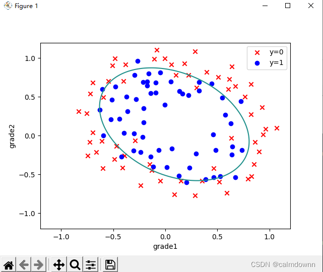
10.预测正确率
这个函数和第一个任务的没有区别
# 预测正确率(实质就是看推测出来的theta值与给定数值的正确率)
def predic_fuc(x, y, theta):
    ct = 0
    t = 0
    p_lst = []
    p_range = sigmode(x @ theta)  # 先将h(x)预测出来的矩阵放入p_range中,里面都是0-1范围的值
    # 循环判断p_range每一行的值,与0.5进行比较,大于等于就默认为被录取,设为1,相反设为0,这些全部存入p_lst列表中
    for i in p_range:
        if i >= 0.5:
            p_lst.append(1)
        elif i < 0.5:
            p_lst.append(0)
    # 将p_lst中预测的值循环与y矩阵中给定的值进行比较,求出相同的次数
    while True:
        if p_lst[t] == y[t]:
            ct += 1
        t += 1
        if t == len(x):
            break
    return ct / len(x)  # 返回预测准确的占总数的百分比
    pass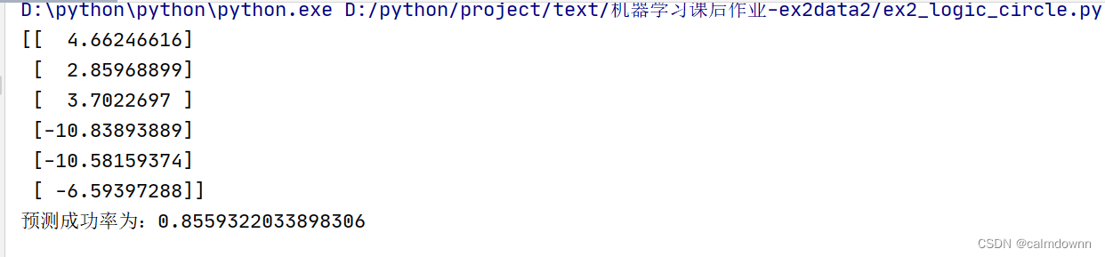
四.全部代码
import numpy as np
import pandas as pd
import matplotlib.pyplot as plt

# 先取出数据
data = pd.read_csv('ex2data2.txt', names=['grade1', 'grade2', 'is_commmitted'])


# 将数据归一化
# data = (data - data.mean()) / data.std()
# data.insert(0, 'ones', 1)  # 在头部插入一列1
# x = data.iloc[:, 0:3]  # 行全要,x获取前三列
# y = data.iloc[:, 3:4]  # 行全要,y获取最后一列
# # 将x,y转换为矩阵
# x = np.matrix(x)
# y = np.matrix(y)
# theta = np.matrix(np.zeros((6, 1)))  # 初始化theta为一个3*1维的矩阵


def feature_mapping(x1, x2):
    data = {}
    data['F10'] = x1
    data['F01'] = x2
    data['F20'] = np.power(x1, 2)
    data['F02'] = np.power(x2, 2)
    data['F11'] = x1 * x2
    return pd.DataFrame(data)


x1 = data['grade1']
x2 = data['grade2']
data2 = feature_mapping(x1, x2)
data2.insert(0, 'ones', 1)
x_new = np.matrix(data2.iloc[:, :])
y = np.matrix(data.iloc[:, 2:3])
theta = np.matrix(np.zeros((6, 1)))


# print(np.shape(x_new))


# 预测的函数h(x)
def sigmode(z):
    return 1 / (1 + np.exp(-z))  # np.exp()在这里将矩阵的每一个值都进行了e为底的变化


# 代价函数
def cost_fuc(x, y, theta, lameda):
    cost_y1 = -(np.log(sigmode(x @ theta)).T @ y)  # 第一部分公式
    cost_y0 = -(np.log(1 - (sigmode(x @ theta))).T @ (1 - y))  # 第二部分公式
    regulate_part = np.sum(np.power(theta, 2)) * (lameda / (2 * len(x)))  # 正则化的一项
    return (cost_y1 + cost_y0) / len(x) + regulate_part
    pass


# print(cost_fuc())  # 看一下初始代价函数

# 梯度下降算法
def gradient_decent(x, y, theta, alpha, update_times, lameda):
    cost_list = []
    for i in range(update_times):
        theta = theta * (1 - (lameda / len(x)) * alpha) - (alpha / len(x)) * (x.T @ (sigmode(x @ theta) - y))
        cost = cost_fuc(x, y, theta, lameda)
        cost_list.append(cost)
    return theta, cost_list
    pass


# lameda = 0.01
# alpha = 0.003


# 边界图
def boudary_line(theta):
    x = np.linspace(-1.2, 1.2, 200)
    xx, yy = np.meshgrid(x, x)
    z = feature_mapping(xx.ravel(), yy.ravel())
    z.insert(0,'ones',1)
    z = np.matrix(z)
    zz = z @ theta
    zz = zz.reshape(xx.shape)
    fig, ax = plt.subplots()
    ax.scatter(data[data['is_commmitted'] == 0]['grade1'], data[data['is_commmitted'] == 0]['grade2'], c='r',
               marker='x',
               label='y=0')
    ax.scatter(data[data['is_commmitted'] == 1]['grade1'], data[data['is_commmitted'] == 1]['grade2'], c='b',
               marker='o',
               label='y=1')
    ax.legend()
    ax.set_xlabel('grade1')
    ax.set_ylabel('grade2')
    plt.contour(xx, yy, zz, 0)
    plt.show()


# 散点图
def scatter_pic():
    positive = data[data['is_commmitted'].isin([1])]  # 找出所有录取结果为1的所有行
    negative = data[data['is_commmitted'].isin([0])]  # 找出所有录取结果为0的所有行
    # 下面是散点图
    fig, ax = plt.subplots(figsize=(12, 8))
    # positive[grade1]就是在所有录取结果为1的行中取出grade1那一列的数据为x轴,并且结果为1的行中grade2为y轴
    ax.scatter(x=positive['grade1'], y=positive['grade2'], color='purple', marker='o', label='committed')
    # positive[grade1]就是在所有录取结果为0的行中取出grade1那一列的数据为x轴,并且结果为0的行中grade2为y轴
    ax.scatter(x=negative['grade1'], y=negative['grade2'], color='orange', marker='x', label='not_committed')
    plt.legend()  # 图例的位置
    ax.set_xlabel('grade1')  # 设置x轴的标题
    ax.set_ylabel('grade1')  # 设置y轴的标题
    plt.show()
    pass

# print(scatter_pic())

# 预测正确率(实质就是看推测出来的theta值与给定数值的正确率)
def predic_fuc(x, y, theta):
    ct = 0
    t = 0
    p_lst = []
    p_range = sigmode(x @ theta)  # 先将h(x)预测出来的矩阵放入p_range中,里面都是0-1范围的值
    # 循环判断p_range每一行的值,与0.5进行比较,大于等于就默认为被录取,设为1,相反设为0,这些全部存入p_lst列表中
    for i in p_range:
        if i >= 0.5:
            p_lst.append(1)
        elif i < 0.5:
            p_lst.append(0)
    # 将p_lst中预测的值循环与y矩阵中给定的值进行比较,求出相同的次数
    while True:
        if p_lst[t] == y[t]:
            ct += 1
        t += 1
        if t == len(x):
            break
    return ct / len(x)  # 返回预测准确的占总数的百分比
    pass


# 预测函数的大致图像
def hx_pic():
    x = np.arange(-10, 10, 0.01)  # x轴-10到10,间隔0.01
    y = sigmode(x)
    plt.plot(x, y, c='r', linestyle='dashdot', label='$g(Z)$')  # 设置x,y坐标,颜色,画线风格,标签
    plt.xlabel('z')  # x轴标签
    plt.ylabel('hx')  # y轴标签
    plt.legend(loc='best')  # 画线的标签位置
    plt.show()

theta1, cost_list = gradient_decent(x_new, y, theta, 0.03, 200000,0.01)
print(theta1)
print(f'预测成功率为:{predic_fuc(x_new, y, theta1)}')
boudary_line(theta1)