补充:特征归一化,意义、方法、使用场景
一:单变量线性回归
(一)导入需要使用的包
import numpy as np
import pandas as pd
import matplotlib.pyplot as plt
(二)导入数据集
注意:一定要将数据文件放在和程序同一个文件夹中,否则要使用绝对路径访问文件。
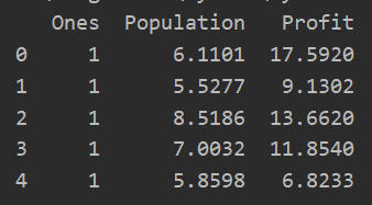
将csv文件读入并转化为数据框DataFrame形式,需要知道路径,指定哪一行作为表头,默认为0,即甚至第一行作为表头,若没有表头,则设置参数header=None,并主动指定列的名称,用列表表示,来添加列名。


6.1101,17.592
5.5277,9.1302
8.5186,13.662
7.0032,11.854
5.8598,6.8233
8.3829,11.886
7.4764,4.3483
8.5781,12
6.4862,6.5987
5.0546,3.8166
5.7107,3.2522
14.164,15.505
5.734,3.1551
8.4084,7.2258
5.6407,0.71618
5.3794,3.5129
6.3654,5.3048
5.1301,0.56077
6.4296,3.6518
7.0708,5.3893
6.1891,3.1386
20.27,21.767
5.4901,4.263
6.3261,5.1875
5.5649,3.0825
18.945,22.638
12.828,13.501
10.957,7.0467
13.176,14.692
22.203,24.147
5.2524,-1.22
6.5894,5.9966
9.2482,12.134
5.8918,1.8495
8.2111,6.5426
7.9334,4.5623
8.0959,4.1164
5.6063,3.3928
12.836,10.117
6.3534,5.4974
5.4069,0.55657
6.8825,3.9115
11.708,5.3854
5.7737,2.4406
7.8247,6.7318
7.0931,1.0463
5.0702,5.1337
5.8014,1.844
11.7,8.0043
5.5416,1.0179
7.5402,6.7504
5.3077,1.8396
7.4239,4.2885
7.6031,4.9981
6.3328,1.4233
6.3589,-1.4211
6.2742,2.4756
5.6397,4.6042
9.3102,3.9624
9.4536,5.4141
8.8254,5.1694
5.1793,-0.74279
21.279,17.929
14.908,12.054
18.959,17.054
7.2182,4.8852
8.2951,5.7442
10.236,7.7754
5.4994,1.0173
20.341,20.992
10.136,6.6799
7.3345,4.0259
6.0062,1.2784
7.2259,3.3411
5.0269,-2.6807
6.5479,0.29678
7.5386,3.8845
5.0365,5.7014
10.274,6.7526
5.1077,2.0576
5.7292,0.47953
5.1884,0.20421
6.3557,0.67861
9.7687,7.5435
6.5159,5.3436
8.5172,4.2415
9.1802,6.7981
6.002,0.92695
5.5204,0.152
5.0594,2.8214
5.7077,1.8451
7.6366,4.2959
5.8707,7.2029
5.3054,1.9869
8.2934,0.14454
13.394,9.0551
5.4369,0.61705
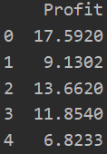
path = 'ex1data1.txt'
data = pd.read_csv(path,header=None,names=['Population','Profit'])
data.head() #数据预览

data.describe() #查看数据描述,包括计数,平均值,标准差,最大最小值,分位数...

(三)数据可视化
data.plot(kind='scatter',x='Population',y="Profit",figsize=(12,8))
plt.show()
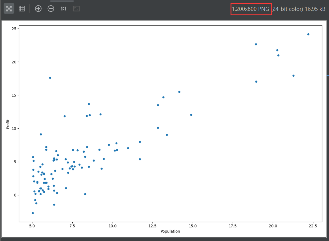
由图可知,数据集存在一定的线性关系。
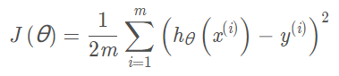
(四)创建代价函数
首先,我们将创建一个以参数θ为特征函数的代价函数
![]()
def computeCost(X,y,theta): #输入X是列向量,y也是列向量,theta是行向量
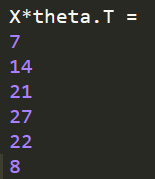
inner = np.power(((X*theta.T)-y),2) #X乘以theta的转置就是假设函数
return np.sum(inner)/(2*len(X)) #求得代价函数
举例:

(五)虽说我们是单变量线性回归,但是我们还是存在一个x_0,全为1,使得我们存在一个常数θ_0
因此,我们需要在训练集中添加一列x_0,以便我们可以使用向量化的解决方案来计算代价和梯度。在训练集左侧插入一列全为1的列,以便计算。
即设置x_0=1,loc=0,name=ones,values=1.
data.insert(0,'Ones',1)
(六)进行变量初始化
cols = data.shape[1]    #获取列数   shape[0]是行数
X = data.iloc[:,0:cols-1]   #获取数据集
y = data.iloc[:,cols-1:cols]    #获取标签值---目标变量
观察X训练集和y目标变量是否正确:
原始数据data: X数据集: y目标变量:


(七)代价函数中传参X,y应该是numpy矩阵,才可以直接计算
由(六)中获取的数据类型是DataFrame类型,因此,我们需要进行类型转换。同时还需要初始化theta,即把theta所有元素都设置为0
X = np.matrix(X.values)
y = np.matrix(y.values)
theta = np.matrix(np.array([0,0]))  #theta是一个(1,2)矩阵

代价函数测试:
computeCost(X,y,theta)
![]()
(八)批量梯度下降
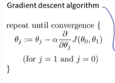
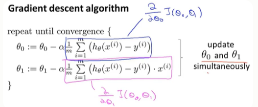
当x_0=1时,两个式子可以合并
def gradientDescennt(X,y,theta,alpha,iters):    #iters是迭代次数 alpha是步长
    temp = np.matrix(np.zeros(theta.shape)) #构建零值矩阵,暂存theta
    parameters = int(theta.ravel().shape[1])    #ravel计算需要求解的参数个数   功能将多维数组降至一维
    cost = np.zeros(iters) #构建iters个0的数组

    for i in range(iters):  #进行迭代
        error = (X*theta.T)-y   #获取差值
        for j in range(parameters): #更新theta_j
            term = np.multiply(error,X[:,j])    #乘以x_i  因为x_0等于1,所以这个式包含theta_0,theta_1
            temp[0,j] = theta[0,j] - (alpha/len(X))*np.sum(term)    #更新theta_j

        theta = temp    #更新全部theta值
        cost[i] = computeCost(X,y,theta)    #更新代价值

    return theta, cost
这里设置:步长alpha = 0.01 迭代次数iters = 1000
g,cost = gradientDescennt(X,y,theta,alpha,iters)    #获取迭代后的theta值,和代价最小值

print(g,cost[-1])  #cost[-1]就是我们最后的最小代价值

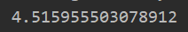
(九)可以用我们拟合过的theta值---g,计算训练模型的代价参数(可以省略)
computeCost(X,y,g)
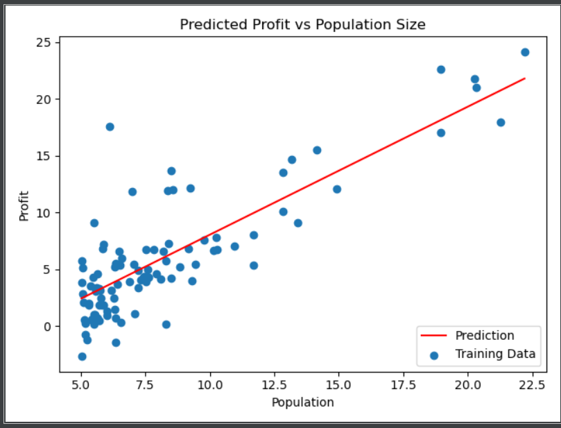
(十)绘制线性模型以及数据,观察拟合程度
#进行绘图
x = np.linspace(data.Population.min(),data.Population.max(),100)    #抽取100个样本
f = g[0,0]+(g[0,1]*x)   #线性函数,利用x抽取的等距样本绘制线性直线

fig, ax = plt.subplots(figsize=(12,8))    #返回图表以及图表相关的区域,为空代表绘制区域为111--->一行一列图表,选中第一个
ax.plot(x,f,'r',label="Prediction") #绘制直线
ax.scatter(data.Population,data.Profit,label='Training Data')    #绘制散点图
ax.legend(loc=4)    #显示标签位置  给图加上图例  'lower right'  : 4,
ax.set_xlabel("Population")
ax.set_ylabel("Profit")
ax.set_title("Predicted Profit vs Population Size")
plt.show()
绘制代价图---代价总是降低的:
fig, ax = plt.subplots()    #返回图表以及图表相关的区域,为空代表绘制区域为111--->一行一列图表,选中第一个
ax.plot(np.arange(iters),cost,'r')
ax.set_xlabel('Iterations')
ax.set_ylabel('Cost')
ax.set_title("Error vs. Training Epoch")
plt.show()

(十一)全部代码
import numpy as np
import pandas as pd
import matplotlib.pyplot as plt

def computeCost(X,y,theta): #输入X是列向量,y也是列向量,theta是行向量
    inner = np.power(((X*theta.T)-y),2) #X乘以theta的转置就是假设函数
    return np.sum(inner)/(2*len(X)) #求得代价函数

def gradientDescennt(X,y,theta,alpha,iters):    #iters是迭代次数
    temp = np.matrix(np.zeros(theta.shape)) #构建零值矩阵,暂存theta
    parameters = int(theta.ravel().shape[1])    #ravel计算需要求解的参数个数   功能将多维数组降至一维
    cost = np.zeros(iters) #构建iters个0的数组

    for i in range(iters):  #进行迭代
        error = (X*theta.T)-y   #获取差值
        for j in range(parameters): #更新theta_j
            term = np.multiply(error,X[:,j])    #乘以x_i  因为x_0等于1,所以这个式包含theta_0,theta_1
            temp[0,j] = theta[0,j] - (alpha/len(X))*np.sum(term)    #更新theta_j

        theta = temp    #更新全部theta值
        cost[i] = computeCost(X,y,theta)    #更新代价值

    return theta, cost

path = 'E:\Python\MachineLearning\ex1data1.txt'
data = pd.read_csv(path,header=None,names=['Population','Profit'])
data.insert(0,'Ones',1)

cols = data.shape[1]    #获取列数   shape[0]是行数
X = data.iloc[:,0:cols-1]   #获取数据集
y = data.iloc[:,cols-1:cols]    #获取标签值---目标变量

X = np.matrix(X.values)
y = np.matrix(y.values)
theta = np.matrix(np.array([0,0]))

alpha = 0.01
iters = 1000

g,cost = gradientDescennt(X,y,theta,alpha,iters)    #获取迭代后的theta值,和代价最小值

#进行绘图
fig, ax = plt.subplots()    #返回图表以及图表相关的区域,为空代表绘制区域为111--->一行一列图表,选中第一个
ax.plot(np.arange(iters),cost,'r')
ax.set_xlabel('Iterations')
ax.set_ylabel('Cost')
ax.set_title("Error vs. Training Epoch")
plt.show()
# x = np.linspace(data.Population.min(),data.Population.max(),100)    #抽取100个样本
# f = g[0,0]+(g[0,1]*x)   #线性函数,利用x抽取的等距样本绘制线性直线
#
# fig, ax = plt.subplots()    #返回图表以及图表相关的区域,为空代表绘制区域为111--->一行一列图表,选中第一个
# ax.plot(x,f,'r',label="Prediction") #绘制直线
# ax.scatter(data.Population,data.Profit,label='Training Data')    #绘制散点图
# ax.legend(loc=4)    #显示标签位置
# ax.set_xlabel("Population")
# ax.set_ylabel("Profit")
# ax.set_title("Predicted Profit vs Population Size")
# plt.show()

# print(g,cost[-1])
# print(computeCost(X,y,g))
# data.plot(kind='scatter',x='Population',y="Profit",figsize=(12,8))
# plt.show()
二:多变量线性回归
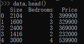
该练习包括一个房屋价格数据集,其中包含两个变量(房屋大小、卧室数量)和目标(房子价格)。
2104,3,399900
1600,3,329900
2400,3,369000
1416,2,232000
3000,4,539900
1985,4,299900
1534,3,314900
1427,3,198999
1380,3,212000
1494,3,242500
1940,4,239999
2000,3,347000
1890,3,329999
4478,5,699900
1268,3,259900
2300,4,449900
1320,2,299900
1236,3,199900
2609,4,499998
3031,4,599000
1767,3,252900
1888,2,255000
1604,3,242900
1962,4,259900
3890,3,573900
1100,3,249900
1458,3,464500
2526,3,469000
2200,3,475000
2637,3,299900
1839,2,349900
1000,1,169900
2040,4,314900
3137,3,579900
1811,4,285900
1437,3,249900
1239,3,229900
2132,4,345000
4215,4,549000
2162,4,287000
1664,2,368500
2238,3,329900
2567,4,314000
1200,3,299000
852,2,179900
1852,4,299900
1203,3,239500
(一)读取数据
path = 'E:\Python\MachineLearning\ex1data2.txt'
data = pd.read_csv(path,header=None,names=['Size','Bedrooms','Price'])
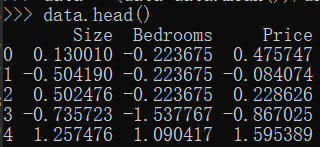
(二)特征归一化(新增预处理步骤)
有时不同特征之间数组的绝对值差距比较大。10000+,0.000+导致数值较大的将数值较小的特征掩盖掉,并且会影响算法收敛的速度。
这里采用标准差标准化: x =(x - u)/σ u是均值 σ是标准差
data = (data-data.mean())/data.std()
(三)其他步骤同一,需要修改维度
def computeCost(X,y,theta): #输入X是列向量,y也是列向量,theta是行向量
    inner = np.power(((X*theta.T)-y),2) #X乘以theta的转置就是假设函数
    return np.sum(inner)/(2*len(X)) #求得代价函数

def gradientDescennt(X,y,theta,alpha,iters):    #iters是迭代次数
    temp = np.matrix(np.zeros(theta.shape)) #构建零值矩阵,暂存theta
    parameters = int(theta.ravel().shape[1])    #ravel计算需要求解的参数个数   功能将多维数组降至一维
    cost = np.zeros(iters) #构建iters个0的数组

    for i in range(iters):  #进行迭代
        error = (X*theta.T)-y   #获取差值
        for j in range(parameters): #更新theta_j
            term = np.multiply(error,X[:,j])    #乘以x_i  因为x_0等于1,所以这个式包含theta_0,theta_1
            temp[0,j] = theta[0,j] - (alpha/len(X))*np.sum(term)    #更新theta_j

        theta = temp    #更新全部theta值
        cost[i] = computeCost(X,y,theta)    #更新代价值

    return theta, cost
data.insert(0,'Ones',1)

cols = data.shape[1]    #获取列数   shape[0]是行数
X = data.iloc[:,0:cols-1]   #获取数据集
y = data.iloc[:,cols-1:cols]    #获取标签值---目标变量

X = np.matrix(X.values)
y = np.matrix(y.values)
theta = np.matrix(np.array([0,0,0]))

alpha = 0.01
iters = 1000

g,cost = gradientDescennt(X,y,theta,alpha,iters)    #获取迭代后的theta值,和代价最小值
(四)查看代价函数收敛图
#进行绘图
fig, ax = plt.subplots()    #返回图表以及图表相关的区域,为空代表绘制区域为111--->一行一列图表,选中第一个
ax.plot(np.arange(iters),cost,'r')
ax.set_xlabel('Iterations')
ax.set_ylabel('Cost')
ax.set_title("Error vs. Training Epoch")
plt.show()

多变量也是随着迭代次数的增加,他的训练误差也是逐渐减小。
三:补充正规方程求θ
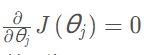
(一)求解θ
正规方程是通过求解下面的方程来找出使得代价函数最小的参数的:
假设我们的训练集特征矩阵为 X(包含了x_0=1)并且我们的训练集结果为向量 y,则利用正规方程解出向量 θ:
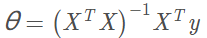
上标T代表矩阵转置,上标-1 代表矩阵的逆。

(二)梯度下降与正规方程的比较:
梯度下降:
需要选择学习率α,需要多次迭代,当特征数量n大时也能较好适用,适用于各种类型的模型
正规方程:
不需要选择学习率α,一次计算得出,需要计算![]() ,如果特征数量n较大则运算代价大,因为矩阵逆的计算时间复杂度为O(n3),通常来说当n小于10000 时还是可以接受的,只适用于线性模型,不适合逻辑回归模型等其他模型
,如果特征数量n较大则运算代价大,因为矩阵逆的计算时间复杂度为O(n3),通常来说当n小于10000 时还是可以接受的,只适用于线性模型,不适合逻辑回归模型等其他模型
![]()
# 正规方程
def normalEqn(X, y):
    theta = np.linalg.inv(X.T@X)@X.T@y#X.T@X等价于X.T.dot(X)
    return theta
final_theta2=normalEqn(X, y)#感觉和批量梯度下降的theta的值有点差距
final_theta2
梯度下降得到的结果是matrix([[-3.24140214, 1.1272942 ]])和上面得到的值有出入。