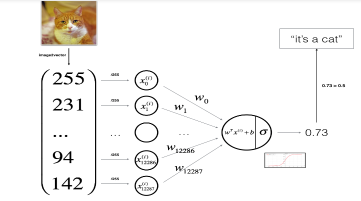
非常推荐大家去学习一下coursera上的DeepLearning.ai课程,Week2的作业是实现逻辑回归算法,细节不再赘述,主要看1张图(逻辑回归算法识别猫和非猫的图片的架构图)和实现的公式(公式要好好理解,看下到底是怎么通过梯度下降来最小化损失函数的,这可以说是最简单的公式了)
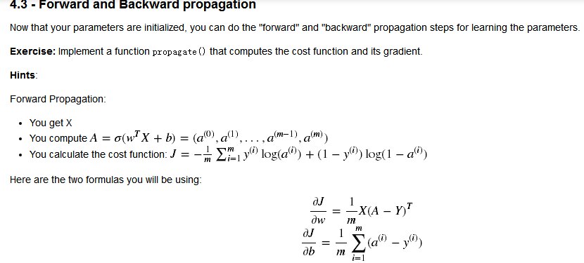
用到的公式:

以下代码可以很好的帮助理解前向传播、反向传播以及梯度下降来学习参数的原理,做完后,我是从Jupyter的notebook上保存下来,稍微修改后的py文件,可以直接在python3 IDE下运行,请安装必要的package,
import numpy as np
import matplotlib.pyplot as plt
import h5py
import scipy
from PIL import Image
from scipy import ndimage
from lr_utils import load_dataset
#get_ipython().magic('matplotlib inline')
train_set_x_orig, train_set_y, test_set_x_orig, test_set_y, classes = load_dataset()
# Example of a picture
index =11
plt.imshow(train_set_x_orig[index])#随便显示训练样本中的一幅图片
print ("y = " + str(train_set_y[:, index]) + ", it's a '" + classes[np.squeeze(train_set_y[:, index])].decode("utf-8") + "' picture.")
plt.show()
# Many software bugs in deep learning come from having matrix/vector dimensions that don't fit.
# If you can keep your matrix/vector dimensions straight you will go a long way toward eliminating many bugs.
# - m_train (number of training examples)
# - m_test (number of test examples)
# - num_px (= height = width of a training image)
# Remember that `train_set_x_orig` is a numpy-array of shape (m_train, num_px, num_px, 3). For instance,
#you can access `m_train` by writing `train_set_x_orig.shape[0]`.
m_train = train_set_x_orig.shape[0]
m_test = test_set_x_orig.shape[0]
num_px = train_set_x_orig.shape[1]
print ("Number of training examples: m_train = " + str(m_train))
print ("Number of testing examples: m_test = " + str(m_test))
print ("Height/Width of each image: num_px = " + str(num_px))
print ("Each image is of size: (" + str(num_px) + ", " + str(num_px) + ", 3)")
print ("train_set_x shape: " + str(train_set_x_orig.shape))
print ("train_set_y shape: " + str(train_set_y.shape))
print ("test_set_x shape: " + str(test_set_x_orig.shape))
print ("test_set_y shape: " + str(test_set_y.shape))
print("------------------------------------------------------------------------------")
# A trick when you want to flatten a matrix X of shape (a,b,c,d) to a matrix X_flatten of shape (b$*$c$*$d, a) is to use:
# ```python
# X_flatten = X.reshape(X.shape[0], -1).T # X.T is the transpose of X
# ```
train_set_x_flatten = train_set_x_orig.reshape(train_set_x_orig.shape[0],-1).T#把样本数作为列数
test_set_x_flatten = test_set_x_orig.reshape(test_set_x_orig.shape[0],-1).T
print ("train_set_x_flatten shape: " + str(train_set_x_flatten.shape))
print ("train_set_y shape: " + str(train_set_y.shape))
print ("test_set_x_flatten shape: " + str(test_set_x_flatten.shape))
print ("test_set_y shape: " + str(test_set_y.shape))
print ("sanity check after reshaping: " + str(train_set_x_flatten[0:5,0]))
print("------------------------------------------------------------------------------")
# To represent color images, the red, green and blue channels (RGB) must be specified for each pixel,
#and so the pixel value is actually a vector of three numbers ranging from 0 to 255.
#
# One common preprocessing step in machine learning is to center and standardize your dataset,
#meaning that you substract the mean of the whole numpy array from each example,
#and then divide each example by the standard deviation of the whole numpy array.
#But for picture datasets, it is simpler and more convenient
#and works almost as well to just divide every row of the dataset by 255 (the maximum value of a pixel channel).
#
# <!-- During the training of your model, you're going to multiply weights and add biases to some initial inputs in order to observe neuron activations.
#Then you backpropogate with the gradients to train the model.
#But, it is extremely important for each feature to have a similar range such that our gradients don't explode.
#You will see that more in detail later in the lectures. !-->
#
# Let's standardize our dataset.
train_set_x = train_set_x_flatten/255.
test_set_x = test_set_x_flatten/255.
# GRADED FUNCTION: sigmoid
def sigmoid(z):
"""
Compute the sigmoid of z
Arguments:
z -- A scalar or numpy array of any size.
Return:
s -- sigmoid(z)
"""
s = 1/(1+np.exp(-z))#激活函数
return s
print ("sigmoid([0, 2]) = " + str(sigmoid(np.array([0,2]))))
print("------------------------------------------------------------------------------")
def initialize_with_zeros(dim):
"""
This function creates a vector of zeros of shape (dim, 1) for w and initializes b to 0.
Argument:
dim -- size of the w vector we want (or number of parameters in this case)
Returns:
w -- initialized vector of shape (dim, 1)
b -- initialized scalar (corresponds to the bias)
"""
w = np.random.randn(dim,1)
w = w-w
b = 0
assert(w.shape == (dim, 1))#要尽可能的使用assert 这里为检查矩阵大小
assert(isinstance(b, float) or isinstance(b, int))
return w, b
dim = 2#假定w为(2,1)矩阵
w, b = initialize_with_zeros(dim)
print ("w = " + str(w))
print ("b = " + str(b))
print("------------------------------------------------------------------------------")
# GRADED FUNCTION: propagate(前向传播和反向传播)
def propagate(w, b, X, Y):
"""
Implement the cost function and its gradient for the propagation explained above
Arguments:
w -- weights, a numpy array of size (num_px * num_px * 3, 1)
b -- bias, a scalar
X -- data of size (num_px * num_px * 3, number of examples)
Y -- true "label" vector (containing 0 if non-cat, 1 if cat) of size (1, number of examples)
Return:
cost -- negative log-likelihood cost for logistic regression
dw -- gradient of the loss with respect to w, thus same shape as w
db -- gradient of the loss with respect to b, thus same shape as b
Tips:
- Write your code step by step for the propagation. np.log(), np.dot()
"""
m = X.shape[1]
# FORWARD PROPAGATION (FROM X TO COST)
A = 1/(1+np.exp(-(np.dot(w.T,X) + b))) # compute activation
cost =-(np.sum(Y*np.log(A)+(1-Y)*np.log(1-A)))/m # compute cost
# BACKWARD PROPAGATION (TO FIND GRAD)
dw =np.dot(X,(A-Y).T)/m
db =np.sum(A-Y)/m
assert(dw.shape == w.shape)
assert(db.dtype == float)
cost = np.squeeze(cost)
assert(cost.shape == ())
grads = {"dw": dw,
"db": db}
return grads, cost
w, b, X, Y = np.array([[1.],[2.]]), 2., np.array([[1.,2.,-1.],[3.,4.,-3.2]]), np.array([[1,0,1]])
grads, cost = propagate(w, b, X, Y)
print ("dw = " + str(grads["dw"]))
print ("db = " + str(grads["db"]))
print ("cost = " + str(cost))
print("------------------------------------------------------------------------------")
# GRADED FUNCTION: optimize
def optimize(w, b, X, Y, num_iterations, learning_rate, print_cost = False):
"""
This function optimizes w and b by running a gradient descent algorithm
Arguments:
w -- weights, a numpy array of size (num_px * num_px * 3, 1)
b -- bias, a scalar
X -- data of shape (num_px * num_px * 3, number of examples)
Y -- true "label" vector (containing 0 if non-cat, 1 if cat), of shape (1, number of examples)
num_iterations -- number of iterations of the optimization loop
learning_rate -- learning rate of the gradient descent update rule
print_cost -- True to print the loss every 100 steps
Returns:
params -- dictionary containing the weights w and bias b
grads -- dictionary containing the gradients of the weights and bias with respect to the cost function
costs -- list of all the costs computed during the optimization, this will be used to plot the learning curve.
Tips:
You basically need to write down two steps and iterate through them:
1) Calculate the cost and the gradient for the current parameters. Use propagate().
2) Update the parameters using gradient descent rule for w and b.
"""
costs = []
for i in range(num_iterations):
# Cost and gradient calculation (≈ 1-4 lines of code)
### START CODE HERE ###
grads, cost = propagate(w, b, X, Y)
### END CODE HERE ###
# Retrieve derivatives from grads
dw = grads["dw"]
db = grads["db"]
# update rule (≈ 2 lines of code)
### START CODE HERE ###
w = w-learning_rate*dw
b = b-learning_rate*db
### END CODE HERE ###
# Record the costs
if i % 100 == 0:
costs.append(cost)
# Print the cost every 100 training examples
if print_cost and i % 100 == 0:
print ("Cost after iteration %i: %f" %(i, cost))
params = {"w": w,
"b": b}
grads = {"dw": dw,
"db": db}
return params, grads, costs
params, grads, costs = optimize(w, b, X, Y, num_iterations= 100, learning_rate = 0.009, print_cost = False)
print ("w = " + str(params["w"]))
print ("b = " + str(params["b"]))
print ("dw = " + str(grads["dw"]))
print ("db = " + str(grads["db"]))
print("------------------------------------------------------------------------------")
# GRADED FUNCTION: predict
def predict(w, b, X):
'''
Predict whether the label is 0 or 1 using learned logistic regression parameters (w, b)
Arguments:
w -- weights, a numpy array of size (num_px * num_px * 3, 1)
b -- bias, a scalar
X -- data of size (num_px * num_px * 3, number of examples)
Returns:
Y_prediction -- a numpy array (vector) containing all predictions (0/1) for the examples in X
'''
m = X.shape[1]
Y_prediction = np.zeros((1,m))
w = w.reshape(X.shape[0], 1)
# Compute vector "A" predicting the probabilities of a cat being present in the picture
A = 1/(1+np.exp(-(np.dot(w.T,X)+b)))
for i in range(A.shape[1]):
# Convert probabilities A[0,i] to actual predictions p[0,i]
if(A[0,i]>0.5):
Y_prediction[0,i] = 1
else:
Y_prediction[0,i] = 0
assert(Y_prediction.shape == (1, m))
return Y_prediction
w = np.array([[0.1124579],[0.23106775]])
b = -0.3
X = np.array([[1.,-1.1,-3.2],[1.2,2.,0.1]])
print ("predictions = " + str(predict(w, b, X)))
print("------------------------------------------------------------------------------")
# GRADED FUNCTION: model
def model(X_train, Y_train, X_test, Y_test, num_iterations = 2000, learning_rate = 0.5, print_cost = False):
"""
Builds the logistic regression model by calling the function you've implemented previously
Arguments:
X_train -- training set represented by a numpy array of shape (num_px * num_px * 3, m_train)
Y_train -- training labels represented by a numpy array (vector) of shape (1, m_train)
X_test -- test set represented by a numpy array of shape (num_px * num_px * 3, m_test)
Y_test -- test labels represented by a numpy array (vector) of shape (1, m_test)
num_iterations -- hyperparameter representing the number of iterations to optimize the parameters
learning_rate -- hyperparameter representing the learning rate used in the update rule of optimize()
print_cost -- Set to true to print the cost every 100 iterations
Returns:
d -- dictionary containing information about the model.
"""
# initialize parameters with zeros (≈ 1 line of code)
w, b = initialize_with_zeros(X_train.shape[0])
# Gradient descent (≈ 1 line of code)
parameters, grads, costs = optimize(w, b, X_train, Y_train, num_iterations, learning_rate, print_cost = False)
# Retrieve parameters w and b from dictionary "parameters"
w = parameters["w"]
b = parameters["b"]
# Predict test/train set examples (≈ 2 lines of code)
Y_prediction_test = predict(w, b, X_test)
Y_prediction_train = predict(w, b, X_train)
# Print train/test Errors
print("train accuracy: {} %".format(100 - np.mean(np.abs(Y_prediction_train - Y_train)) * 100))
print("test accuracy: {} %".format(100 - np.mean(np.abs(Y_prediction_test - Y_test)) * 100))
d = {"costs": costs,
"Y_prediction_test": Y_prediction_test,
"Y_prediction_train" : Y_prediction_train,
"w" : w,
"b" : b,
"learning_rate" : learning_rate,
"num_iterations": num_iterations}
return d
# Run the following cell to train your model.
d = model(train_set_x, train_set_y, test_set_x, test_set_y, num_iterations = 2000, learning_rate = 0.005, print_cost = True)
print("------------------------------------------------------------------------------")
# Example of a picture that was wrongly classified.
index =2
#plt.imshow(test_set_x[:,index].reshape((num_px, num_px, 3)))
#print ("y = " + str(test_set_y[0,index]) + ", you predicted that it is a \"" + classes[d["Y_prediction_test"][0,index]].decode("utf-8") + "\" picture.")
# Plot learning curve (with costs)
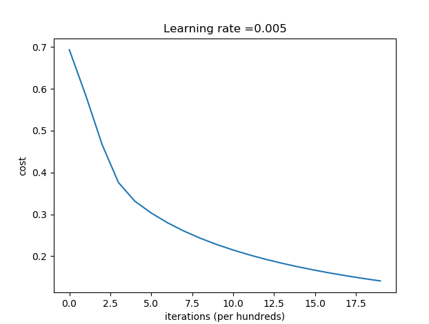
costs = np.squeeze(d['costs'])
plt.plot(costs)
plt.ylabel('cost')
plt.xlabel('iterations (per hundreds)')
plt.title("Learning rate =" + str(d["learning_rate"]))
plt.show()
my_image = "C:\\Users\\Desktop\\image\\22.jpg" # change this to the name of your image file
# We preprocess the image to fit your algorithm.
fname = my_image
image = np.array(ndimage.imread(fname, flatten=False))
my_image = scipy.misc.imresize(image, size=(num_px,num_px)).reshape((1, num_px*num_px*3)).T
my_predicted_image = predict(d["w"], d["b"], my_image)
plt.imshow(image)
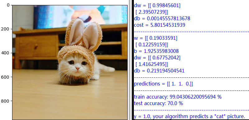
print("y = " + str(np.squeeze(my_predicted_image)) + ", your algorithm predicts a \"" + classes[int(np.squeeze(my_predicted_image)),].decode("utf-8") + "\" picture.")
plt.show()最终结果如下:
Number of training examples: m_train = 209
Number of testing examples: m_test = 50
Height/Width of each image: num_px = 64
Each image is of size: (64, 64, 3)
train_set_x shape: (209, 64, 64, 3)
train_set_y shape: (1, 209)
test_set_x shape: (50, 64, 64, 3)
test_set_y shape: (1, 50)
------------------------------------------------------------------------------
train_set_x_flatten shape: (12288, 209)
train_set_y shape: (1, 209)
test_set_x_flatten shape: (12288, 50)
test_set_y shape: (1, 50)
sanity check after reshaping: [17 31 56 22 33]
------------------------------------------------------------------------------
sigmoid([0, 2]) = [ 0.5 0.88079708]
------------------------------------------------------------------------------
w = [[ 0.]
[ 0.]]
b = 0
------------------------------------------------------------------------------
dw = [[ 0.99845601]
[ 2.39507239]]
db = 0.00145557813678
cost = 5.80154531939
------------------------------------------------------------------------------
w = [[ 0.19033591]
[ 0.12259159]]
b = 1.92535983008
dw = [[ 0.67752042]
[ 1.41625495]]
db = 0.219194504541
------------------------------------------------------------------------------
predictions = [[ 1. 1. 0.]]
------------------------------------------------------------------------------
train accuracy: 99.04306220095694 %
test accuracy: 70.0 %(因为采用的是最基础的学习模型,然后样本不多,所以准确率也不高)
识别自己的图片(虽然是最简单的逻辑回归算法,然后这个待耳朵的猫咪,照样识别了出来!):