吴恩达深度学习 第二课第一周编程作业_Gradient Checking（梯度检查）

Gradient Checking 梯度检查

声明

本文作业是在jupyter notebook上一步一步做的，带有一些过程中查找的资料等（出处已标明）并翻译成了中文，如有错误，欢迎指正！

参考：https://blog.csdn.net/u013733326/article/details/79847918

参考Kulbear 的 【Initialization】和【Regularization】 和 【Gradient Checking】，以及念师的【10. 初始化、正则化、梯度检查实战】，以及何宽 ，

---

欢迎来到本周的期末作业！在这项作业中，你将学习如何实现和使用渐变检查。
你是一个团队的一员，致力于全球范围内的移动支付，并被要求建立一个深度学习模型来检测欺诈行为——每当有人进行支付时，你都想看看支付是否有欺诈行为，比如用户的账户是否被黑客占领。
但是反向传播的实现相当具有挑战性，有时还存在缺陷。因为这是一个任务关键型应用程序，所以您公司的首席执行官希望确定您的反向传播实现是正确的。你的首席执行官说，“给我一个证据，证明你的反向传播是有效的！”为了保证这一点，您将使用“梯度检查”。
开始吧！

# Packages
import numpy as np
from testCases import *
from gc_utils import sigmoid, relu, dictionary_to_vector, vector_to_dictionary, gradients_to_vector

1) How does gradient checking work?  梯度检查是如何工作的？

反向传播计算梯度，其中θ表示模型的参数。使用前向传播和损失函数计算 J，因为前向传播相对容易实现，所以您确信自己是正确的，因此您几乎百分之百确定您正确地计算了成本J。因此，您可以使用计算J的代码来验证用于计算的代码。

让我们回顾一下导数（或梯度）的定义：

如果你不熟悉“limε→0”表示法，那只是表示“当ε真的很小时”

我们知道以下几点：

•是你想要确保你计算正确的东西。

•您可以计算J（θ+ε）和J（θ-ε）（在θ是实数的情况下），因为您确信J的实现是正确的。

让我们用等式（1）和一个小的ε值来说服您的CEO，您用于计算的代码是正确的！

2) 1-dimensional gradient checking 一维梯度检查

考虑一维线性函数J（θ）=θx，该模型仅包含一个实值参数θ，以x为输入。
您将实现计算J（.）及其导数的代码。然后使用梯度检查来确保J的导数计算是正确的。

**Figure 1** : **1D linear model** 图一 一维线性模型

上图显示了关键的计算步骤：首先从x开始，然后计算函数J（x）（“前向传播”）。然后计算导数（“反向传播”）。

练习：为这个简单函数实现“正向传播”和“反向传播”。一、 在两个不同的函数中计算J（.）（“前向传播”）及其相对于θ的导数（“反向传播”）

 1 # GRADED FUNCTION: forward_propagation
 2 
 3 def forward_propagation(x, theta):
 4     """
 5     Implement the linear forward propagation (compute J) presented in Figure 1 (J(theta) = theta * x)
 6     
 7     Arguments:
 8     x -- a real-valued input
 9     theta -- our parameter, a real number as well
10     
11     Returns:
12     J -- the value of function J, computed using the formula J(theta) = theta * x
13     """
14     
15     ### START CODE HERE ### (approx. 1 line)
16     J = theta * x
17     ### END CODE HERE ###
18     
19     return J

# GRADED FUNCTION: forward_propagation

x, theta = 2, 4
J = forward_propagation(x, theta)
print ("J = " + str(J))

练习：现在，实现图1中的反向传播步骤（导数计算）。也就是说，计算J（θ）=θx相对于θ的导数。为了省去做微积分，你应该得到dtheta==x。

 1 # GRADED FUNCTION: backward_propagation
 2 
 3 def backward_propagation(x, theta):
 4     """
 5     Computes the derivative of J with respect to theta (see Figure 1).
 6     
 7     Arguments:
 8     x -- a real-valued input
 9     theta -- our parameter, a real number as well
10     
11     Returns:
12     dtheta -- the gradient of the cost with respect to theta 相对于θ的成本梯度
13     """
14     
15     ### START CODE HERE ### (approx. 1 line)
16     dtheta = x
17     ### END CODE HERE ###
18     
19     return dtheta

# GRADED FUNCTION: backward_propagation

x, theta = 2, 4
dtheta = backward_propagation(x, theta)
print ("dtheta = " + str(dtheta))

练习：为了证明反向传播函数正确地计算了梯度，让我们实现梯度检查。
说明：

•首先使用上述公式（1）和较小的ε值计算“gradeapprox”。以下是要遵循的步骤：

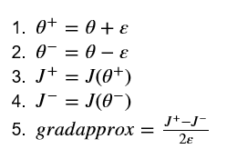
•然后使用反向传播计算梯度，并将结果存储在变量“grad”中

•最后，使用以下公式计算“gradeapprow”和“grad”之间的相对差：

计算此公式需要3个步骤：

1、使用np.linalg.norm(...)计算分子

2、计算分母。你需要使用np.linalg.norm（…）两次。

3、把他们相除

•如果这个差异很小（比如小于10^-7），您可以非常确信您已经正确地计算了梯度。否则，梯度计算可能会出错。

 1 # GRADED FUNCTION: gradient_check
 2 
 3 def gradient_check(x, theta, epsilon = 1e-7):
 4     """
 5     Implement the backward propagation presented in Figure 1.
 6     
 7     Arguments:
 8     x -- a real-valued input
 9     theta -- our parameter, a real number as well
10     epsilon -- tiny shift to the input to compute approximated gradient with formula(1)
11     
12     Returns:
13     difference -- difference (2) between the approximated gradient and the backward propagation gradient近似梯度和后向传播梯度之间的差异
14     """
15     
16     # Compute gradapprox using left side of formula (1). epsilon is small enough, you don't need to worry about the limit.
17     ### START CODE HERE ### (approx. 5 lines)
18     thetaplus = theta + epsilon                             # Step 1
19     thetaminus = theta - epsilon                              # Step 2
20     J_plus = forward_propagation(x, thetaplus)                                 # Step 3
21     J_minus = forward_propagation(x, thetaminus)                               # Step 4
22     gradapprox =  (J_plus - J_minus) / (2 * epsilon)                            # Step 5
23     ### END CODE HERE ###
24     
25     # Check if gradapprox is close enough to the output of backward_propagation() 检查gradapprox是否足够接近backward_propagation（）的输出
26     ### START CODE HERE ### (approx. 1 line)
27     grad = backward_propagation(x, theta)
28     ### END CODE HERE ###
29     
30     ### START CODE HERE ### (approx. 1 line)
31     numerator =  np.linalg.norm(grad - gradapprox)                            # Step 1'
32     denominator = np.linalg.norm(grad) + np.linalg.norm(gradapprox)                            # Step 2'
33     difference = numerator / denominator                             # Step 3'
34     ### END CODE HERE ###
35     
36     if difference < 1e-7:
37         print ("The gradient is correct!")
38     else:
39         print ("The gradient is wrong!")
40     
41     return difference

# GRADED FUNCTION: gradient_check

x, theta = 2, 4
difference = gradient_check(x, theta)
print("difference = " + str(difference))

结果：

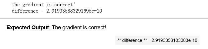
恭喜你，误差小于10-7阈值。因此，您可以有很高的信心，您已经正确地计算了反向传播（）中的梯度。
现在，在更一般的情况下，成本函数J有不止一个一维输入。当你训练一个神经网络时，θ实际上由多个矩阵W^[l]和偏差b^[l]组成！重要的是要知道如何使用高维输入进行梯度检查。开始吧！

3) N-dimensional gradient checking N维梯度检查

下图描述了欺诈检测模型的正向和反向传播。高维参数是怎样计算的呢？我们看一下下图：

**Figure 2** : **deep neural network** 图2 深度神经网络
*LINEAR -> RELU -> LINEAR -> RELU -> LINEAR -> SIGMOID*

让我们来看看您的前向传播和后向传播的实现。

 1 def forward_propagation_n(X, Y, parameters):
 2     """
 3     Implements the forward propagation (and computes the cost) presented in Figure 3.
 4     
 5     Arguments:
 6     X -- training set for m examples
 7     Y -- labels for m examples 
 8     parameters -- python dictionary containing your parameters "W1", "b1", "W2", "b2", "W3", "b3":包含参数“W1”，“b1”，“W2”，“b2”，“W3”，“b3”的python字典：
 9                     W1 -- weight matrix of shape (5, 4)权重矩阵，维度为（5,4）
10                     b1 -- bias vector of shape (5, 1)偏向量，维度为（5,1）
11                     W2 -- weight matrix of shape (3, 5)
12                     b2 -- bias vector of shape (3, 1)
13                     W3 -- weight matrix of shape (1, 3)
14                     b3 -- bias vector of shape (1, 1)
15     
16     Returns:
17     cost -- the cost function (logistic cost for one example) - 成本函数（logistic）
18     """
19     
20     # retrieve parameters
21     m = X.shape[1]
22     W1 = parameters["W1"]
23     b1 = parameters["b1"]
24     W2 = parameters["W2"]
25     b2 = parameters["b2"]
26     W3 = parameters["W3"]
27     b3 = parameters["b3"]
28 
29     # LINEAR -> RELU -> LINEAR -> RELU -> LINEAR -> SIGMOID
30     Z1 = np.dot(W1, X) + b1
31     A1 = relu(Z1)
32     Z2 = np.dot(W2, A1) + b2
33     A2 = relu(Z2)
34     Z3 = np.dot(W3, A2) + b3
35     A3 = sigmoid(Z3)
36 
37     # Cost
38     logprobs = np.multiply(-np.log(A3),Y) + np.multiply(-np.log(1 - A3), 1 - Y)
39     cost = 1./m * np.sum(logprobs)
40     
41     cache = (Z1, A1, W1, b1, Z2, A2, W2, b2, Z3, A3, W3, b3)
42     
43     return cost, cache

现在，运行反向传播。

 1 def backward_propagation_n(X, Y, cache):
 2     """
 3     Implement the backward propagation presented in figure 2.
 4     
 5     Arguments:
 6     X -- input datapoint, of shape (input size, 1) 输入数据点（输入节点数量，1）
 7     Y -- true "label"标签
 8     cache -- cache output from forward_propagation_n() 来自forward_propagation_n（）的cache输出
 9     
10     Returns:
11     gradients -- A dictionary with the gradients of the cost with respect to each parameter, activation and pre-activation variables. 一个字典，其中包含与每个参数、激活和激活前变量相关的成本梯度。
12     """
13     
14     m = X.shape[1]
15     (Z1, A1, W1, b1, Z2, A2, W2, b2, Z3, A3, W3, b3) = cache
16     
17     dZ3 = A3 - Y
18     dW3 = 1./m * np.dot(dZ3, A2.T)
19     db3 = 1./m * np.sum(dZ3, axis=1, keepdims = True)
20     
21     dA2 = np.dot(W3.T, dZ3)
22     dZ2 = np.multiply(dA2, np.int64(A2 > 0))
23     dW2 = 1./m * np.dot(dZ2, A1.T)
24     db2 = 1./m * np.sum(dZ2, axis=1, keepdims = True)
25     
26     dA1 = np.dot(W2.T, dZ2)
27     dZ1 = np.multiply(dA1, np.int64(A1 > 0))
28     dW1 = 1./m * np.dot(dZ1, X.T)
29     db1 = 1./m * np.sum(dZ1, axis=1, keepdims = True)
30     
31     gradients = {"dZ3": dZ3, "dW3": dW3, "db3": db3,
32                  "dA2": dA2, "dZ2": dZ2, "dW2": dW2, "db2": db2,
33                  "dA1": dA1, "dZ1": dZ1, "dW1": dW1, "db1": db1}
34     
35     return gradients

您在欺诈检测测试集上获得了一些结果，但您对您的模型没有100%的把握。没有人是完美的！让我们实现梯度检查来验证梯度是否正确。

梯度检查是如何工作的？

如1）和2）中所述，您需要将“gradeapproach”与反向传播计算的梯度进行比较。公式仍然是：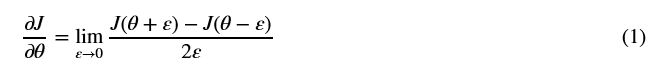

然而，θ不再是标量。这是一本叫做“参数”的字典。我们为您实现了一个函数“dictionary_to_vector（）”。它将“parameters”字典转换为一个名为“values”的向量，该向量通过将所有参数（W1、b1、W2、b2、W3、b3）重塑为向量并将它们连接起来而获得。反函数是“向量字典”，它输出“参数”字典。

**Figure 2** : **dictionary_to_vector() and vector_to_dictionary()**
You will need these functions in gradient_check_n()

我们还使用gradients_to_vector（）将“gradients”字典转换为向量“grad”。你不用担心这个。
练习：实现梯度检查。
说明：下面是一些伪代码，可以帮助您实现梯度检查。
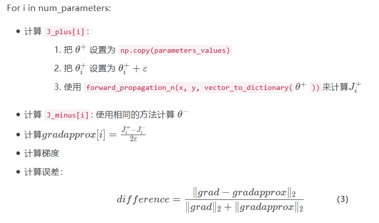
对于每个i in num_参数：

 1 # GRADED FUNCTION: gradient_check_n
 2 
 3 def gradient_check_n(parameters, gradients, X, Y, epsilon = 1e-7):
 4     """
 5     Checks if backward_propagation_n computes correctly the gradient of the cost output by forward_propagation_n
 6     检查backward_propagation_n是否正确计算forward_propagation_n输出的成本梯度
 7     
 8     Arguments:
 9     parameters -- python dictionary containing your parameters "W1", "b1", "W2", "b2", "W3", "b3": parameters - 包含参数“W1”，“b1”，“W2”，“b2”，“W3”，“b3”的python字典：
10     grad -- output of backward_propagation_n, contains gradients of the cost with respect to the parameters.grad_output_propagation_n的输出包含与参数相关的成本梯度。 
11     x -- input datapoint, of shape (input size, 1)
12     y -- true "label"
13     epsilon -- tiny shift to the input to compute approximated gradient with formula(1) 计算输入的微小偏移以计算近似梯度
14     
15     Returns:
16     difference -- difference (2) between the approximated gradient and the backward propagation gradient
17     """
18     
19     # Set-up variables 设置变量
20     parameters_values, _ = dictionary_to_vector(parameters) #这边keys用不到，可以用“_”代替
21     grad = gradients_to_vector(gradients)
22     num_parameters = parameters_values.shape[0]
23     J_plus = np.zeros((num_parameters, 1))
24     J_minus = np.zeros((num_parameters, 1))
25     gradapprox = np.zeros((num_parameters, 1))
26     
27     # Compute gradapprox
28     for i in range(num_parameters):
29         
30         # Compute J_plus[i]. Inputs: "parameters_values, epsilon". Output = "J_plus[i]".计算J_plus [i]。输入：“parameters_values，epsilon”。输出=“J_plus [i]”
31         # "_" is used because the function you have to outputs two parameters but we only care about the first one
32         ### START CODE HERE ### (approx. 3 lines)
33         thetaplus =  np.copy(parameters_values)                          # Step 1
34         thetaplus[i][0] = thetaplus[i][0] + epsilon                             # Step 2
35         J_plus[i], _ = forward_propagation_n(X, Y, vector_to_dictionary(thetaplus))                                # Step 3
36         ### END CODE HERE ###
37         
38         # Compute J_minus[i]. Inputs: "parameters_values, epsilon". Output = "J_minus[i]".
39         ### START CODE HERE ### (approx. 3 lines)
40         thetaminus = np.copy(parameters_values)                                  # Step 1
41         thetaminus[i][0] =  thetaminus[i][0] - epsilon                            # Step 2        
42         J_minus[i], _ = forward_propagation_n(X, Y, vector_to_dictionary(thetaminus))                # Step 3
43         ### END CODE HERE ###
44         
45         # Compute gradapprox[i]
46         ### START CODE HERE ### (approx. 1 line)
47         gradapprox[i] = (J_plus[i] - J_minus[i]) / (2. * epsilon)
48         ### END CODE HERE ###
49     
50     # Compare gradapprox to backward propagation gradients by computing difference.
51     ### START CODE HERE ### (approx. 1 line)
52     numerator = np.linalg.norm(grad - gradapprox)                                       # Step 1'
53     denominator = np.linalg.norm(grad) + np.linalg.norm(gradapprox)            # Step 2'
54     difference = numerator / denominator                                     # Step 3'
55     ### END CODE HERE ###
56 
57     if difference > 1e-7:
58         print ("\033[93m" + "There is a mistake in the backward propagation! difference = " + str(difference) + "\033[0m")
59     else:
60         print ("\033[92m" + "Your backward propagation works perfectly fine! difference = " + str(difference) + "\033[0m")
61     
62     return difference

# GRADED FUNCTION: gradient_check_n

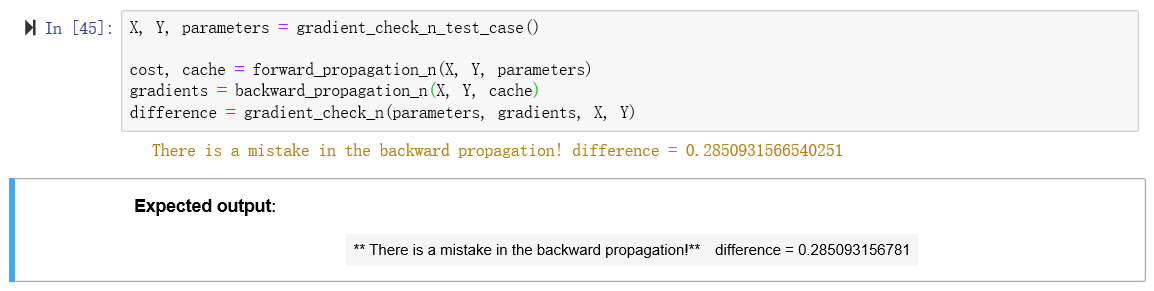
X, Y, parameters = gradient_check_n_test_case()

cost, cache = forward_propagation_n(X, Y, parameters)
gradients = backward_propagation_n(X, Y, cache)
difference = gradient_check_n(parameters, gradients, X, Y)

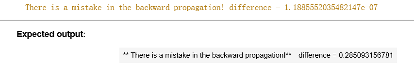
我们给你的反向传播代码似乎有错误！很好，你已经实现了梯度检查。返回反向传播并尝试查找/更正错误（提示：检查dW2和db1）。当你认为你已经修复了梯度检查。请记住，如果修改代码，则需要重新执行定义反向传播的单元格。
你能用梯度检查来证明你的导数计算正确吗？即使作业的这一部分没有评分，我们强烈建议您尝试找到错误并重新运行渐变检查，直到您确信backprop现在已经正确实现。

 

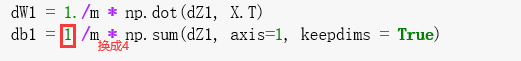
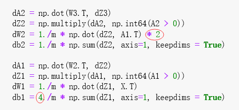
 修改后：

Note：

梯度检查很慢！用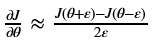近似梯度计算成本很高。由于这个原因，我们不在训练期间的每次迭代中运行梯度检查。只需几次检查梯度是否正确。

梯度检查，至少我们已经介绍过了，对dropout不起作用。你通常会运行梯度检查算法没有辍学，以确保你的backprop是正确的，然后添加辍学。
恭喜你，你可以相信你的深度学习模型是正确的！你甚至可以用这个来说服你的CEO。:)
**你应该记住这本笔记本**:-梯度检查 验证了 反向传播的梯度 和 梯度的数值近似（使用正向传播计算）之间  的  接近度。

梯度检查很慢，所以我们不是在每次训练迭代中都运行它。您通常只运行它以确保您的代码是正确的，然后关闭它并使用backprop进行实际的学习过程。