改善深层神经网络第一周-Gradient Checking（梯度检查）

Gradient Checking

Welcome to the final assignment for this week! In this assignment you will learn to implement and use gradient checking.

You are part of a team working to make mobile payments available globally, and are asked to build a deep learning model to detect fraud–whenever someone makes a payment, you want to see if the payment might be fraudulent, such as if the user’s account has been taken over by a hacker. (你是全球范围内开展移动支付的团队的一部分，并被要求建立一个深度学习模式来检测欺诈行为 - 每当有人付款时，你想要查看付款是否有欺诈行为，例如用户帐户已被黑客占用。)

But backpropagation is quite challenging to implement, and sometimes has bugs. Because this is a mission-critical application, your company’s CEO wants to be really certain that your implementation of backpropagation is correct. Your CEO says, “Give me a proof that your backpropagation is actually working!” To give this reassurance, you are going to use “gradient checking”.(* 

但是反向传播实施起来相当具有挑战性，有时会有错误。因为这是关键任务应用程序，所以贵公司的首席执行官要真正确定你的反向传播实施是正确的。你的首席执行官说：“给我一个证明你的反向传播实际上是有效的！”为了让这个保证，你将使用“梯度检查”。*)

# Packages
import numpy as np
from testCases import *
from gc_utils import sigmoid, relu, dictionary_to_vector, vector_to_dictionary, gradients_to_vector

其中testCases的代码如下：

# -*- coding: utf-8 -*-
"""
Created on Sun Apr 22 12:57:30 2018

@author: StephenGai
"""
import numpy as np

def compute_cost_with_regularization_test_case():
    np.random.seed(1)
    Y_assess = np.array([[1, 1, 0, 1, 0]])
    W1 = np.random.randn(2, 3)
    b1 = np.random.randn(2, 1)
    W2 = np.random.randn(3, 2)
    b2 = np.random.randn(3, 1)
    W3 = np.random.randn(1, 3)
    b3 = np.random.randn(1, 1)
    parameters = {"W1": W1, "b1": b1, "W2": W2, "b2": b2, "W3": W3, "b3": b3}
    a3 = np.array([[ 0.40682402,  0.01629284,  0.16722898,  0.10118111,  0.40682402]])
    return a3, Y_assess, parameters

def backward_propagation_with_regularization_test_case():
    np.random.seed(1)
    X_assess = np.random.randn(3, 5)
    Y_assess = np.array([[1, 1, 0, 1, 0]])
    cache = (np.array([[-1.52855314,  3.32524635,  2.13994541,  2.60700654, -0.75942115],
         [-1.98043538,  4.1600994 ,  0.79051021,  1.46493512, -0.45506242]]),
  np.array([[ 0.        ,  3.32524635,  2.13994541,  2.60700654,  0.        ],
         [ 0.        ,  4.1600994 ,  0.79051021,  1.46493512,  0.        ]]),
  np.array([[-1.09989127, -0.17242821, -0.87785842],
         [ 0.04221375,  0.58281521, -1.10061918]]),
  np.array([[ 1.14472371],
         [ 0.90159072]]),
  np.array([[ 0.53035547,  5.94892323,  2.31780174,  3.16005701,  0.53035547],
         [-0.69166075, -3.47645987, -2.25194702, -2.65416996, -0.69166075],
         [-0.39675353, -4.62285846, -2.61101729, -3.22874921, -0.39675353]]),
  np.array([[ 0.53035547,  5.94892323,  2.31780174,  3.16005701,  0.53035547],
         [ 0.        ,  0.        ,  0.        ,  0.        ,  0.        ],
         [ 0.        ,  0.        ,  0.        ,  0.        ,  0.        ]]),
  np.array([[ 0.50249434,  0.90085595],
         [-0.68372786, -0.12289023],
         [-0.93576943, -0.26788808]]),
  np.array([[ 0.53035547],
         [-0.69166075],
         [-0.39675353]]),
  np.array([[-0.3771104 , -4.10060224, -1.60539468, -2.18416951, -0.3771104 ]]),
  np.array([[ 0.40682402,  0.01629284,  0.16722898,  0.10118111,  0.40682402]]),
  np.array([[-0.6871727 , -0.84520564, -0.67124613]]),
  np.array([[-0.0126646]]))
    return X_assess, Y_assess, cache

def forward_propagation_with_dropout_test_case():
    np.random.seed(1)
    X_assess = np.random.randn(3, 5)
    W1 = np.random.randn(2, 3)
    b1 = np.random.randn(2, 1)
    W2 = np.random.randn(3, 2)
    b2 = np.random.randn(3, 1)
    W3 = np.random.randn(1, 3)
    b3 = np.random.randn(1, 1)
    parameters = {"W1": W1, "b1": b1, "W2": W2, "b2": b2, "W3": W3, "b3": b3}
    
    return X_assess, parameters

def backward_propagation_with_dropout_test_case():
    np.random.seed(1)
    X_assess = np.random.randn(3, 5)
    Y_assess = np.array([[1, 1, 0, 1, 0]])
    cache = (np.array([[-1.52855314,  3.32524635,  2.13994541,  2.60700654, -0.75942115],
           [-1.98043538,  4.1600994 ,  0.79051021,  1.46493512, -0.45506242]]), np.array([[ True, False,  True,  True,  True],
           [ True,  True,  True,  True, False]], dtype=bool), np.array([[ 0.        ,  0.        ,  4.27989081,  5.21401307,  0.        ],
           [ 0.        ,  8.32019881,  1.58102041,  2.92987024,  0.        ]]), np.array([[-1.09989127, -0.17242821, -0.87785842],
           [ 0.04221375,  0.58281521, -1.10061918]]), np.array([[ 1.14472371],
           [ 0.90159072]]), np.array([[ 0.53035547,  8.02565606,  4.10524802,  5.78975856,  0.53035547],
           [-0.69166075, -1.71413186, -3.81223329, -4.61667916, -0.69166075],
           [-0.39675353, -2.62563561, -4.82528105, -6.0607449 , -0.39675353]]), np.array([[ True, False,  True, False,  True],
           [False,  True, False,  True,  True],
           [False, False,  True, False, False]], dtype=bool), np.array([[ 1.06071093,  0.        ,  8.21049603,  0.        ,  1.06071093],
           [ 0.        ,  0.        ,  0.        ,  0.        ,  0.        ],
           [ 0.        ,  0.        ,  0.        ,  0.        ,  0.        ]]), np.array([[ 0.50249434,  0.90085595],
           [-0.68372786, -0.12289023],
           [-0.93576943, -0.26788808]]), np.array([[ 0.53035547],
           [-0.69166075],
           [-0.39675353]]), np.array([[-0.7415562 , -0.0126646 , -5.65469333, -0.0126646 , -0.7415562 ]]), np.array([[ 0.32266394,  0.49683389,  0.00348883,  0.49683389,  0.32266394]]), np.array([[-0.6871727 , -0.84520564, -0.67124613]]), np.array([[-0.0126646]]))


    return X_assess, Y_assess, cache

def gradient_check_n_test_case(): 
    np.random.seed(1)
    x = np.random.randn(4,3)
    y = np.array([1, 1, 0])
    W1 = np.random.randn(5,4) 
    b1 = np.random.randn(5,1) 
    W2 = np.random.randn(3,5) 
    b2 = np.random.randn(3,1) 
    W3 = np.random.randn(1,3) 
    b3 = np.random.randn(1,1) 
    parameters = {"W1": W1,
                  "b1": b1,
                  "W2": W2,
                  "b2": b2,
                  "W3": W3,
                  "b3": b3}

    
    return x, y, parameters

gc_utils的代码如下：（需要注意形成字典的那个函数）

# -*- coding: utf-8 -*-
"""
Created on Sun Apr 22 18:21:39 2018

@author: StephenGai
"""
import numpy as np

def sigmoid(x):
    """
    Compute the sigmoid of x

    Arguments:
    x -- A scalar or numpy array of any size.

    Return:
    s -- sigmoid(x)
    """
    s = 1/(1+np.exp(-x))
    return s

def relu(x):
    """
    Compute the relu of x

    Arguments:
    x -- A scalar or numpy array of any size.

    Return:
    s -- relu(x)
    """
    s = np.maximum(0,x)
    
    return s

def dictionary_to_vector(parameters):
    """
    Roll all our parameters dictionary into a single vector satisfying our specific required shape.
    """
    keys = []
    count = 0
    for key in ["W1", "b1", "W2", "b2", "W3", "b3"]:      
        # flatten parameter
        new_vector = np.reshape(parameters[key], (-1,1))
        keys = keys + [key]*new_vector.shape[0]
        
        if count == 0:
            theta = new_vector
        else:
            theta = np.concatenate((theta, new_vector), axis=0)
        count = count + 1

    return theta, keys

def vector_to_dictionary(theta):
    """
    Unroll all our parameters dictionary from a single vector satisfying our specific required shape.
    """
    parameters = {}
    parameters["W1"] = theta[:20].reshape((5,4))
    parameters["b1"] = theta[20:25].reshape((5,1))
    parameters["W2"] = theta[25:40].reshape((3,5))
    parameters["b2"] = theta[40:43].reshape((3,1))
    parameters["W3"] = theta[43:46].reshape((1,3))
    parameters["b3"] = theta[46:47].reshape((1,1))

    return parameters

def gradients_to_vector(gradients):
    """
    Roll all our gradients dictionary into a single vector satisfying our specific required shape.
    """
    count = 0
    for key in ["dW1", "db1", "dW2", "db2", "dW3", "db3"]:
        # flatten parameter
        new_vector = np.reshape(gradients[key], (-1,1))
        
        if count == 0:
            theta = new_vector
        else:
            theta = np.concatenate((theta, new_vector), axis=0)
        count = count + 1

    return theta

Backpropagation computes the gradients $\frac{\partial J}{\partial \theta }$, where $\theta$ denotes the parameters of the model. $J$ is computed using forward propagation and your loss function.(反向传播计算梯度$\frac{\partial J}{\partial \theta }$，其中$\theta$表示模型的参数。 $J$是使用正向传播和损失函数来计算的。)

Because forward propagation is relatively easy to implement, you’re confident you got that right, and so you’re almost 100% sure that you’re computing the cost $J$ correctly. Thus, you can use your code for computing $J$ to verify the code for computing $\frac{\partial \mathrm{J/}}{\partial \theta }$. (由于向前传播相对容易实现，所以你确信自己得到了正确的结果，所以你几乎100％肯定你正在计算成本$J$。因此，你可以使用你的代码来计算$J$来验证计算$\frac{\partial \mathrm{J/}}{\partial \theta }$的代码。)

Let’s look back at the definition of a derivative (or gradient)(倒数或者梯度的定义): 

                            

If you’re not familiar with the “$\underset{\epsilon \to 0}{lim}$” notation, it’s just a way of saying “when $\epsilon$ is really really small.”

We know the following:

• $\frac{\partial J}{\partial \theta }$ is what you want to make sure you’re computing correctly.
• You can compute $J\left(\theta +\epsilon \right)$ and $J\left(\theta -\epsilon \right)$ (in the case that $\theta$ is a real number), since you’re confident your implementation for $J$ is correct.

Lets use equation (1) and a small value for $\epsilon$ to convince your CEO that your code for computing $\frac{\partial J}{\partial \theta }$ is correct!

2) 1-dimensional gradient checking

Consider a 1D linear function $J\left(\theta \right)=\theta x$. The model contains only a single real-valued parameter $\theta$, and takes $x$ as input.(考虑一维线性函数$J\left(\theta \right)=\theta x$。该模型只包含一个实值参数$\theta$，并将$x$作为输入)

You will implement code to compute $J(.)$ and its derivative $\frac{\partial J}{\partial \theta }$. You will then use gradient checking to make sure your derivative computation for $J$ is correct. (* 
您将实现代码来计算$J(.)$及其派生$\frac{\partial J}{\partial \theta }$。然后，您将使用梯度检查来确保$J$的派生计算是正确的。*)

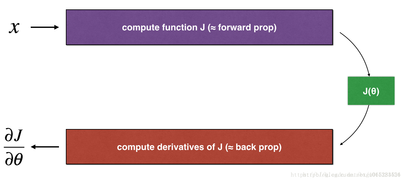
The diagram above shows the key computation steps: First start with $x$, then evaluate the function $J\left(x\right)$ (“forward propagation”). Then compute the derivative $\frac{\partial J}{\partial \theta }$ (“backward propagation”).

Exercise: implement “forward propagation” and “backward propagation” for this simple function. I.e., compute both $J(.)$ (“forward propagation”) and its derivative with respect to $\theta$ (“backward propagation”), in two separate functions.

def forward_propagation(x, theta):
    """
    Implement the linear forward propagation (compute J) presented in Figure 1 (J(theta) = theta * x)

    Arguments:
    x -- a real-valued input
    theta -- our parameter, a real number as well

    Returns:
    J -- the value of function J, computed using the formula J(theta) = theta * x
    """

    ### START CODE HERE ### (approx. 1 line)
    J = np.dot(theta,x)
    ### END CODE HERE ###

    return J

x, theta = 2, 4
J = forward_propagation(x, theta)
print ("J = " + str(J))

运行结果：

J = 8

Expected Output:

def backward_propagation(x, theta):
    """
    Computes the derivative of J with respect to theta (see Figure 1).

    Arguments:
    x -- a real-valued input
    theta -- our parameter, a real number as well

    Returns:
    dtheta -- the gradient of the cost with respect to theta
    """

    ### START CODE HERE ### (approx. 1 line)
    dtheta = x
    ### END CODE HERE ###

    return dtheta
x, theta = 2, 4
dtheta = backward_propagation(x, theta)
print ("dtheta = " + str(dtheta))

运行结果：

dtheta = 2

Exercise : To show that the  backward_propagation()  function is correctly computing the gradient  $\frac{\partial J}{\partial \theta }$

, let’s implement gradient checking.

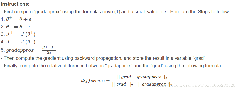
You will need 3 Steps to compute this formula: 
- 1’. compute the numerator using np.linalg.norm(…) 
- 2’. compute the denominator. You will need to call np.linalg.norm(…) twice. 
- 3’. divide them. 
- If this difference is small (say less than ${10}^{-7}$

), you can be quite confident that you have computed your gradient correctly. Otherwise, there may be a mistake in the gradient computation.

def gradient_check(x, theta, epsilon = 1e-7):
    """
    Implement the backward propagation presented in Figure 1.

    Arguments:
    x -- a real-valued input
    theta -- our parameter, a real number as well
    epsilon -- tiny shift to the input to compute approximated gradient with formula(1)

    Returns:
    difference -- difference (2) between the approximated gradient and the backward propagation gradient
    """

    # Compute gradapprox using left side of formula (1). epsilon is small enough, you don't need to worry about the limit.
    ### START CODE HERE ### (approx. 5 lines)
    thetaplus = theta + epsilon                                # Step 1
    thetaminus = theta - epsilon                               # Step 2
    J_plus = forward_propagation(x, thetaplus)                                   # Step 3
    J_minus = forward_propagation(x, thetaminus)                                  # Step 4
    gradapprox = (J_plus - J_minus)/(2*epsilon)                               # Step 5
    ### END CODE HERE ###

    # Check if gradapprox is close enough to the output of backward_propagation()
    ### START CODE HERE ### (approx. 1 line)
    grad = backward_propagation(x, theta) 
    ### END CODE HERE ###

    ### START CODE HERE ### (approx. 1 line)
    numerator = np.linalg.norm(grad - gradapprox)                              # Step 1'
    denominator = np.linalg.norm(grad) + np.linalg.norm(gradapprox)                             # Step 2'
    difference = numerator/denominator                              # Step 3'
    ### END CODE HERE ###

    if difference < 1e-7:
        print ("The gradient is correct!")
    else:
        print ("The gradient is wrong!")

    return difference

x, theta = 2, 4
difference = gradient_check(x, theta)
print("difference = " + str(difference))

输出：

x, theta = 2, 4
difference = gradient_check(x, theta)
print("difference = " + str(difference))

Congrats, the difference is smaller than the ${10}^{-7}$ threshold. So you can have high confidence that you’ve correctly computed the gradient in backward_propagation().

Now, in the more general case, your cost function $J$ has more than a single 1D input. When you are training a neural network, $\theta$ actually consists of multiple matrices $W^{\left[l\right]}$ and biases $b^{\left[l\right]}$! It is important to know how to do a gradient check with higher-dimensional inputs. Let’s do it!

3) N-dimensional gradient checking

The following figure describes the forward and backward propagation of your fraud detection model.

Figure 2 :  deep neural network

LINEAR -> RELU -> LINEAR -> RELU -> LINEAR -> SIGMOID

Let’s look at your implementations for forward propagation and backward propagation.

def forward_propagation_n(X, Y, parameters):
    """
    Implements the forward propagation (and computes the cost) presented in Figure 3.

    Arguments:
    X -- training set for m examples
    Y -- labels for m examples
    parameters -- python dictionary containing your parameters "W1", "b1", "W2", "b2", "W3", "b3":
                    W1 -- weight matrix of shape (5, 4)
                    b1 -- bias vector of shape (5, 1)
                    W2 -- weight matrix of shape (3, 5)
                    b2 -- bias vector of shape (3, 1)
                    W3 -- weight matrix of shape (1, 3)
                    b3 -- bias vector of shape (1, 1)

    Returns:
    cost -- the cost function (logistic cost for one example)
    """

    # retrieve parameters
    m = X.shape[1]
    W1 = parameters["W1"]
    b1 = parameters["b1"]
    W2 = parameters["W2"]
    b2 = parameters["b2"]
    W3 = parameters["W3"]
    b3 = parameters["b3"]

    # LINEAR -> RELU -> LINEAR -> RELU -> LINEAR -> SIGMOID
    Z1 = np.dot(W1, X) + b1
    A1 = relu(Z1)
    Z2 = np.dot(W2, A1) + b2
    A2 = relu(Z2)
    Z3 = np.dot(W3, A2) + b3
    A3 = sigmoid(Z3)

    # Cost
    logprobs = np.multiply(-np.log(A3),Y) + np.multiply(-np.log(1 - A3), 1 - Y)
    cost = 1./m * np.sum(logprobs)

    cache = (Z1, A1, W1, b1, Z2, A2, W2, b2, Z3, A3, W3, b3)

    return cost, cache

Now, run backward propagation.

def backward_propagation_n(X, Y, cache):
    """
    Implement the backward propagation presented in figure 2.

    Arguments:
    X -- input datapoint, of shape (input size, 1)
    Y -- true "label"
    cache -- cache output from forward_propagation_n()

    Returns:
    gradients -- A dictionary with the gradients of the cost with respect to each parameter, activation and pre-activation variables.
    """

    m = X.shape[1]
    (Z1, A1, W1, b1, Z2, A2, W2, b2, Z3, A3, W3, b3) = cache

    dZ3 = A3 - Y
    dW3 = 1./m * np.dot(dZ3, A2.T)
    db3 = 1./m * np.sum(dZ3, axis=1, keepdims = True)

    dA2 = np.dot(W3.T, dZ3)
    dZ2 = np.multiply(dA2, np.int64(A2 > 0))
    dW2 = 1./m * np.dot(dZ2, A1.T)   #不需要乘2
    db2 = 1./m * np.sum(dZ2, axis=1, keepdims = True)

    dA1 = np.dot(W2.T, dZ2)
    dZ1 = np.multiply(dA1, np.int64(A1 > 0))
    dW1 = 1./m * np.dot(dZ1, X.T)
    db1 = 1./m * np.sum(dZ1, axis=1, keepdims = True)   #前面4改为1

    gradients = {"dZ3": dZ3, "dW3": dW3, "db3": db3,
                 "dA2": dA2, "dZ2": dZ2, "dW2": dW2, "db2": db2,
                 "dA1": dA1, "dZ1": dZ1, "dW1": dW1, "db1": db1}

    return gradients

You obtained some results on the fraud detection test set but you are not 100% sure of your model. Nobody’s perfect! Let’s implement gradient checking to verify if your gradients are correct.(你在欺诈检测测试集中获得了一些结果，但你并不是100％确定你的模型。没有人是完美的！让我们实施梯度检查，以验证你的梯度是否正确。)

How does gradient checking work?.

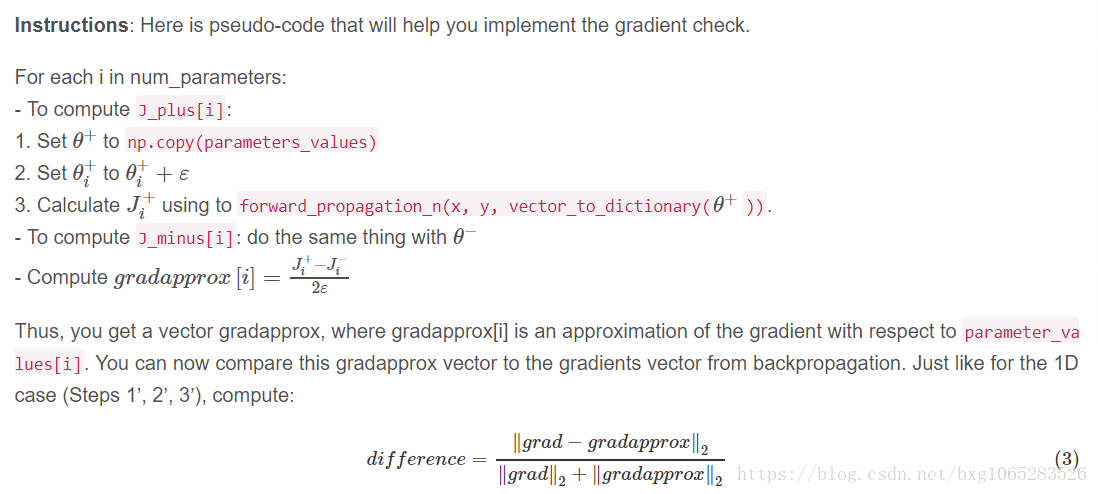
As in 1) and 2), you want to compare “gradapprox” to the gradient computed by backpropagation. The formula is still:

However, $\theta$ is not a scalar anymore. It is a dictionary called “parameters”. We implemented a function “dictionary_to_vector()” for you. It converts the “parameters” dictionary into a vector called “values”, obtained by reshaping all parameters (W1, b1, W2, b2, W3, b3) into vectors and concatenating them.(但是，$\theta$不再是标量了。这是一个名为“参数”的字典。我们为你实现了一个函数“dictionary_to_vector（）”。它将“参数”字典转换成一个称为“值”的向量，通过将所有参数（W1，b1，W2，b2，W3，b3）整形成向量并连接它们而获得。)

The inverse function is “vector_to_dictionary” which outputs back the “parameters” dictionary.

Figure 2 :  dictionary_to_vector() and vector_to_dictionary()
You will need these functions in gradient_check_n()

We have also converted the “gradients” dictionary into a vector “grad” using gradients_to_vector(). You don’t need to worry about that.

Exercise: Implement gradient_check_n().

# GRADED FUNCTION: gradient_check_n

def gradient_check_n(parameters, gradients, X, Y, epsilon = 1e-7):
    """
    Checks if backward_propagation_n computes correctly the gradient of the cost output by forward_propagation_n

    Arguments:
    parameters -- python dictionary containing your parameters "W1", "b1", "W2", "b2", "W3", "b3":
    grad -- output of backward_propagation_n, contains gradients of the cost with respect to the parameters. 
    x -- input datapoint, of shape (input size, 1)
    y -- true "label"
    epsilon -- tiny shift to the input to compute approximated gradient with formula(1)

    Returns:
    difference -- difference (2) between the approximated gradient and the backward propagation gradient
    """

    # Set-up variables
    parameters_values, _ = dictionary_to_vector(parameters)
    grad = gradients_to_vector(gradients)
    num_parameters = parameters_values.shape[0]
    J_plus = np.zeros((num_parameters, 1))
    J_minus = np.zeros((num_parameters, 1))
    gradapprox = np.zeros((num_parameters, 1))

    # Compute gradapprox
    for i in range(num_parameters):

        # Compute J_plus[i]. Inputs: "parameters_values, epsilon". Output = "J_plus[i]".
        # "_" is used because the function you have to outputs two parameters but we only care about the first one
        ### START CODE HERE ### (approx. 3 lines)
        thetaplus = np.copy(parameters_values)                                            # Step 1
        thetaplus[i][0] = thetaplus[i][0] + epsilon                                       # Step 2
        J_plus[i], _ = forward_propagation_n(X, Y, vector_to_dictionary(thetaplus))       # Step 3
        ### END CODE HERE ###

        # Compute J_minus[i]. Inputs: "parameters_values, epsilon". Output = "J_minus[i]".
        ### START CODE HERE ### (approx. 3 lines)
        thetaminus = np.copy(parameters_values)                                           # Step 1
        thetaminus[i][0] = thetaminus[i][0] - epsilon                                     # Step 2        
        J_minus[i], _ = forward_propagation_n(X, Y, vector_to_dictionary(thetaminus))     # Step 3

        ### END CODE HERE ###

        # Compute gradapprox[i]
        ### START CODE HERE ### (approx. 1 line)
        gradapprox[i] =  (J_plus[i] - J_minus[i])/(2*epsilon)
        ### END CODE HERE ###

    # Compare gradapprox to backward propagation gradients by computing difference.
    ### START CODE HERE ### (approx. 1 line)
    numerator = np.linalg.norm(grad - gradapprox)                                         # Step 1'
    denominator = np.linalg.norm(grad) + np.linalg.norm(gradapprox)                       # Step 2'
    difference = numerator/denominator                                                    # Step 3'
    ### END CODE HERE ###

    if difference > 1e-7:
        print ("\033[93m" + "There is a mistake in the backward propagation! difference = " + str(difference) + "\033[0m")
    else:
        print ("\033[92m" + "Your backward propagation works perfectly fine! difference = " + str(difference) + "\033[0m")

    return difference

运行结果：

There is a mistake in the backward propagation! difference = 1.1890913023330276e-07

It seems that there were errors in the backward_propagation_n code we gave you! Good that you’ve implemented the gradient check. Go back to backward_propagation and try to find/correct the errors (Hint: check dW2 and db1). Rerun the gradient check when you think you’ve fixed it. Remember you’ll need to re-execute the cell defining backward_propagation_n() if you modify the code. (看来我们给你的backward_propagation_n代码有错误！很好，你已经实施了梯度检查。返回到backward_propagation并尝试查找/更正错误（提示：检查dW2和db1）。当你认为你已经修复了，重新运行渐变检查。记住，如果修改代码，则需要重新执行定义“backward_propagation_n（）”的单元格。)

Can you get gradient check to declare your derivative computation correct? Even though this part of the assignment isn’t graded, we strongly urge you to try to find the bug and re-run gradient check until you’re convinced backprop is now correctly implemented. (你能得到梯度检查来声明你的派生计算是正确的吗？即使这部分任务没有分级，但我们强烈建议您尝试查找错误并重新运行梯度检查，直到您确信backprop现在已正确实施。)

What you should remember from this notebook: 
- Gradient checking verifies closeness between the gradients from backpropagation and the numerical approximation of the gradient (computed using forward propagation). 
- Gradient checking is slow, so we don’t run it in every iteration of training. You would usually run it only to make sure your code is correct, then turn it off and use backprop for the actual learning process.