吴恩达深度学习第二课第一周作业编程题

声明
本文内容代码都是在【何宽】的【参考教程】基础上，更正了其中的一些错误，只保留了最主要的一些操作步骤。如需了解更详细的信息，还请参考【原文】。

资源获取

点击百度网盘获取，密码为55xd。里面有两个文件夹and三个.py文件，全部解压到你写的代码文件的目录下~

part1——正则化

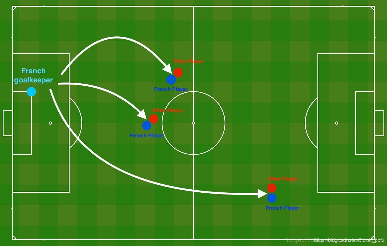
Problem statement：Problem Statement: You have just been hired as an AI expert by the French Football Corporation. They would like you to recommend positions where France’s goal keeper should kick the ball so that the French team’s players can then hit it with their head.

题目陈述

假设你现在是一个AI专家，你需要设计一个模型，可以用于预测在足球场中守门员将球发至哪个位置可以让本队的球员抢到球的可能性更大。

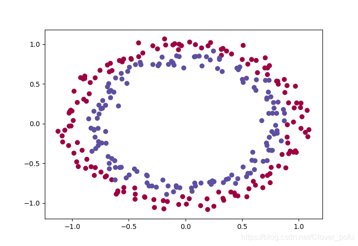
说白了，实际上就是一个二分类，一半是己方抢到球，一半就是对方抢到球。看一下这个图：

自己新建一个.py文件，开始这部分的练习吧~

导入库

import numpy as np
import matplotlib.pyplot as plt
import sklearn
import sklearn.datasets
import reg_utils    #第二部分，正则化

plt.rcParams['figure.figsize'] = (7.0, 4.0) # set default size of plots
plt.rcParams['image.interpolation'] = 'nearest'
plt.rcParams['image.cmap'] = 'gray'

读取并绘制数据

train_X, train_Y, test_X, test_Y = reg_utils.load_2D_dataset(is_plot=True)
plt.show()

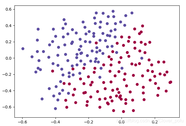
数据看完把is_plot置成False，并删掉plt.show()，以免干扰到后面的图像绘制。

模型函数

def model(X,Y,learning_rate=0.3,num_iterations=30000,print_cost=True,is_plot=True,lambd=0,keep_prob=1):
    grads = {}
    costs = []
    m = X.shape[1]
    layers_dims = [X.shape[0],20,3,1]
    
    #初始化参数
    parameters = reg_utils.initialize_parameters(layers_dims)
    
    #开始学习
    for i in range(0,num_iterations):
        #前向传播
        ##是否随机删除节点
        if keep_prob == 1:
            ###不随机删除节点
            a3 , cache = reg_utils.forward_propagation(X,parameters)
        elif keep_prob < 1:
            ###随机删除节点
            a3 , cache = forward_propagation_with_dropout(X,parameters,keep_prob)
        else:
            print("keep_prob参数错误！程序退出。")
            exit
        
        #计算成本
        ## 是否使用二范数
        if lambd == 0:
            ###不使用L2正则化
            cost = reg_utils.compute_cost(a3,Y)
        else:
            ###使用L2正则化
            cost = compute_cost_with_regularization(a3,Y,parameters,lambd)
        
        #反向传播
        ##可以同时使用L2正则化和随机删除节点，但是本次实验不同时使用。
        assert(lambd == 0  or keep_prob ==1)
        
        ##两个参数的使用情况
        if (lambd == 0 and keep_prob == 1):
            ### 不使用L2正则化和不使用随机删除节点
            grads = reg_utils.backward_propagation(X,Y,cache)
        elif lambd != 0:
            ### 使用L2正则化，不使用随机删除节点
            grads = backward_propagation_with_regularization(X, Y, cache, lambd)
        elif keep_prob < 1:
            ### 使用随机删除节点，不使用L2正则化
            grads = backward_propagation_with_dropout(X, Y, cache, keep_prob)
        
        #更新参数
        parameters = reg_utils.update_parameters(parameters, grads, learning_rate)
        
        #记录并打印成本
        if i % 1000 == 0:
            ## 记录成本
            costs.append(cost)
            if (print_cost and i % 10000 == 0):
                #打印成本
                print("第" + str(i) + "次迭代，成本值为：" + str(cost))
        
    #是否绘制成本曲线图
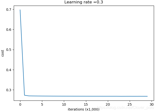
    if is_plot:
        plt.plot(costs)
        plt.ylabel('cost')
        plt.xlabel('iterations (x1,000)')
        plt.title("Learning rate =" + str(learning_rate))
        plt.show()
    
    #返回学习后的参数
    return parameters

不使用正则化

添加以下代码并运行

parameters = model(train_X, train_Y,is_plot=True)
print("训练集:")
predictions_train = reg_utils.predict(train_X, train_Y, parameters)
print("测试集:")
predictions_test = reg_utils.predict(test_X, test_Y, parameters)

plt.title("Model without regularization")
axes = plt.gca()
axes.set_xlim([-0.75,0.40])
axes.set_ylim([-0.75,0.65])
reg_utils.plot_decision_boundary(lambda x: reg_utils.predict_dec(parameters, x.T), train_X, train_Y)

得到的结果如下：

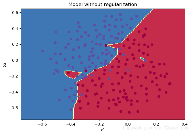
第0次迭代，成本值为：0.6557412523481002
第10000次迭代，成本值为：0.16329987525724213
第20000次迭代，成本值为：0.13851642423265018
训练集:
Accuracy: 0.9478672985781991
测试集:
Accuracy: 0.915

从分类图中看到，出现了过拟合的现象。

使用L2正则化

L2正则化的损失函数

def compute_cost_with_regularization(A3,Y,parameters,lambd):
    m = Y.shape[1]
    W1 = parameters["W1"]
    W2 = parameters["W2"]
    W3 = parameters["W3"]
    
    cross_entropy_cost = reg_utils.compute_cost(A3,Y)
    
    L2_regularization_cost = lambd * (np.sum(np.square(W1)) + np.sum(np.square(W2))  + np.sum(np.square(W3))) / (2 * m)
    
    cost = cross_entropy_cost + L2_regularization_cost
    
    return cost

适用于L2正则化的反向传播函数

def backward_propagation_with_regularization(X, Y, cache, lambd):
    
    m = X.shape[1]
    
    (Z1, A1, W1, b1, Z2, A2, W2, b2, Z3, A3, W3, b3) = cache
    
    dZ3 = A3 - Y
    
    dW3 = (1 / m) * np.dot(dZ3,A2.T) + ((lambd * W3) / m )
    db3 = (1 / m) * np.sum(dZ3,axis=1,keepdims=True)
    
    dA2 = np.dot(W3.T,dZ3)
    dZ2 = np.multiply(dA2,np.int64(A2 > 0))
    dW2 = (1 / m) * np.dot(dZ2,A1.T) + ((lambd * W2) / m)
    db2 = (1 / m) * np.sum(dZ2,axis=1,keepdims=True)
    
    dA1 = np.dot(W2.T,dZ2)
    dZ1 = np.multiply(dA1,np.int64(A1 > 0))
    dW1 = (1 / m) * np.dot(dZ1,X.T) + ((lambd * W1) / m)
    db1 = (1 / m) * np.sum(dZ1,axis=1,keepdims=True)
    
    gradients = {"dZ3": dZ3, "dW3": dW3, "db3": db3, "dA2": dA2,
                 "dZ2": dZ2, "dW2": dW2, "db2": db2, "dA1": dA1, 
                 "dZ1": dZ1, "dW1": dW1, "db1": db1}
    
    return gradients

添加以下代码并运行

parameters = model(train_X, train_Y, lambd=0.7,is_plot=True)
print("使用正则化，训练集:")
predictions_train = reg_utils.predict(train_X, train_Y, parameters)
print("使用正则化，测试集:")
predictions_test = reg_utils.predict(test_X, test_Y, parameters)


plt.title("Model with L2 regularization")
axes = plt.gca()
axes.set_xlim([-0.75,0.40])
axes.set_ylim([-0.75,0.65])
reg_utils.plot_decision_boundary(lambda x: reg_utils.predict_dec(parameters, x.T), train_X, train_Y)

得到的结果如下：

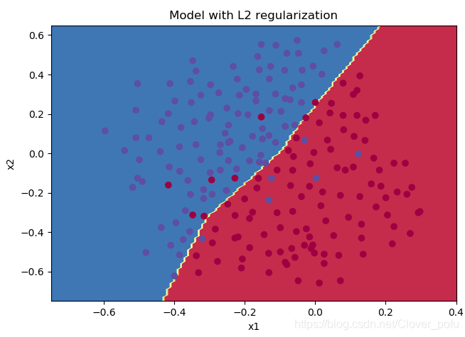
第0次迭代，成本值为：0.6974484493131264
第10000次迭代，成本值为：0.2684918873282239
第20000次迭代，成本值为：0.2680916337127301
使用正则化，训练集:
Accuracy: 0.9383886255924171
使用正则化，测试集:
Accuracy: 0.93

从分类图像看出，过拟合现象消除。分类去掉了一些离群点（错误样本），导致训练集的准确度下降，但测试的准确度上升。

使用Dropout

前向传播函数

def forward_propagation_with_dropout(X,parameters,keep_prob=0.5):
    np.random.seed(1)
    
    W1 = parameters["W1"]
    b1 = parameters["b1"]
    W2 = parameters["W2"]
    b2 = parameters["b2"]
    W3 = parameters["W3"]
    b3 = parameters["b3"]
    
    #LINEAR -> RELU -> LINEAR -> RELU -> LINEAR -> SIGMOID
    Z1 = np.dot(W1,X) + b1
    A1 = reg_utils.relu(Z1)
    
    #下面的步骤1-4对应于上述的步骤1-4。
    D1 = np.random.rand(A1.shape[0],A1.shape[1])    #步骤1：初始化矩阵D1 = np.random.rand(..., ...)
    D1 = D1 < keep_prob                             #步骤2：将D1的值转换为0或1（使​​用keep_prob作为阈值）
    A1 = A1 * D1                                    #步骤3：舍弃A1的一些节点（将它的值变为0或False）
    A1 = A1 / keep_prob                             #步骤4：缩放未舍弃的节点(不为0)的值
    
    Z2 = np.dot(W2,A1) + b2
    A2 = reg_utils.relu(Z2)
    
    #下面的步骤1-4对应于上述的步骤1-4。
    D2 = np.random.rand(A2.shape[0],A2.shape[1])    #步骤1：初始化矩阵D2 = np.random.rand(..., ...)
    D2 = D2 < keep_prob                             #步骤2：将D2的值转换为0或1（使​​用keep_prob作为阈值）
    A2 = A2 * D2                                    #步骤3：舍弃A1的一些节点（将它的值变为0或False）
    A2 = A2 / keep_prob                             #步骤4：缩放未舍弃的节点(不为0)的值
    
    Z3 = np.dot(W3, A2) + b3
    A3 = reg_utils.sigmoid(Z3)
    
    cache = (Z1, D1, A1, W1, b1, Z2, D2, A2, W2, b2, Z3, A3, W3, b3)
    
    return A3, cache

反向传播函数

def backward_propagation_with_dropout(X,Y,cache,keep_prob):
    m = X.shape[1]
    (Z1, D1, A1, W1, b1, Z2, D2, A2, W2, b2, Z3, A3, W3, b3) = cache
    
    dZ3 = A3 - Y
    dW3 = (1 / m) * np.dot(dZ3,A2.T)
    db3 = 1. / m * np.sum(dZ3, axis=1, keepdims=True)
    dA2 = np.dot(W3.T, dZ3)
    
    dA2 = dA2 * D2          # 步骤1：使用正向传播期间相同的节点，舍弃那些关闭的节点（因为任何数乘以0或者False都为0或者False）
    dA2 = dA2 / keep_prob   # 步骤2：缩放未舍弃的节点(不为0)的值
    
    dZ2 = np.multiply(dA2, np.int64(A2 > 0))
    dW2 = 1. / m * np.dot(dZ2, A1.T)
    db2 = 1. / m * np.sum(dZ2, axis=1, keepdims=True)
    
    dA1 = np.dot(W2.T, dZ2)
    
    dA1 = dA1 * D1          # 步骤1：使用正向传播期间相同的节点，舍弃那些关闭的节点（因为任何数乘以0或者False都为0或者False）
    dA1 = dA1 / keep_prob   # 步骤2：缩放未舍弃的节点(不为0)的值

    dZ1 = np.multiply(dA1, np.int64(A1 > 0))
    dW1 = 1. / m * np.dot(dZ1, X.T)
    db1 = 1. / m * np.sum(dZ1, axis=1, keepdims=True)
    
    gradients = {"dZ3": dZ3, "dW3": dW3, "db3": db3,"dA2": dA2,
                 "dZ2": dZ2, "dW2": dW2, "db2": db2, "dA1": dA1, 
                 "dZ1": dZ1, "dW1": dW1, "db1": db1}
    
    return gradients

，我们尝试用keep_prob=0.86来跑一下，添加以下代码并运行

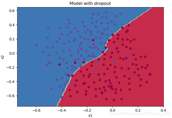
parameters = model(train_X, train_Y, keep_prob=0.86, learning_rate=0.3,is_plot=True)

print("使用随机删除节点，训练集:")
predictions_train = reg_utils.predict(train_X, train_Y, parameters)
print("使用随机删除节点，测试集:")
reg_utils.predictions_test = reg_utils.predict(test_X, test_Y, parameters)

plt.title("Model with dropout")
axes = plt.gca()
axes.set_xlim([-0.75, 0.40])
axes.set_ylim([-0.75, 0.65])
reg_utils.plot_decision_boundary(lambda x: reg_utils.predict_dec(parameters, x.T), train_X, train_Y)

得到以下结果：

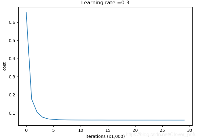
第0次迭代，成本值为：0.6543912405149825
/home/clover/pytorch学习各种测试代码/2_1/reg_utils.py:121: RuntimeWarning: divide by zero encountered in log
  logprobs = np.multiply(-np.log(a3),Y) + np.multiply(-np.log(1 - a3), 1 - Y)
/home/clover/pytorch学习各种测试代码/2_1/reg_utils.py:121: RuntimeWarning: invalid value encountered in multiply
  logprobs = np.multiply(-np.log(a3),Y) + np.multiply(-np.log(1 - a3), 1 - Y)
第10000次迭代，成本值为：0.06101698657490562
第20000次迭代，成本值为：0.060582435798513114
使用随机删除节点，训练集:
Accuracy: 0.9289099526066351
使用随机删除节点，测试集:
Accuracy: 0.95

虽然出现了一些warning，但只要不是error就别怕，能跑就行   (ㅍ_ㅍ)
看来这次dropout效果不错，测试集的准确率达到了95%。好了，关于正则化的测试就到这，下面是梯度爆炸and梯度消失。
 

part2——梯度爆炸或消失

我选择重新建一个.py文件来跑这一部分。

导入库

import numpy as np
import matplotlib.pyplot as plt
import sklearn
import sklearn.datasets
import init_utils   #第一部分，初始化

plt.rcParams['figure.figsize'] = (7.0, 4.0) # set default size of plots
plt.rcParams['image.interpolation'] = 'nearest'
plt.rcParams['image.cmap'] = 'gray'

读取并绘制数据

train_X, train_Y, test_X, test_Y = init_utils.load_dataset(is_plot=True)
plt.show()

运行代码后将会出现以下图样

模型

def model(X,Y,learning_rate=0.01,num_iterations=15000,print_cost=True,initialization="he",is_polt=True):
    grads = {}
    costs = []
    m = X.shape[1]
    layers_dims = [X.shape[0],10,5,1]
    
    #选择初始化参数的类型
    if initialization == "zeros":
        parameters = initialize_parameters_zeros(layers_dims)
    elif initialization == "random":
        parameters = initialize_parameters_random(layers_dims)
    elif initialization == "he":
        parameters = initialize_parameters_he(layers_dims)
    else : 
        print("错误的初始化参数！程序退出")
        exit
    
    #开始学习
    for i in range(0,num_iterations):
        #前向传播
        a3 , cache = init_utils.forward_propagation(X,parameters)
        
        #计算成本        
        cost = init_utils.compute_loss(a3,Y)
        
        #反向传播
        grads = init_utils.backward_propagation(X,Y,cache)
        
        #更新参数
        parameters = init_utils.update_parameters(parameters,grads,learning_rate)
        
        #记录成本
        if i % 1000 == 0:
            costs.append(cost)
            #打印成本
            if print_cost:
                print("第" + str(i) + "次迭代，成本值为：" + str(cost))
        
    
    #学习完毕，绘制成本曲线
    if is_polt:
        plt.plot(costs)
        plt.ylabel('cost')
        plt.xlabel('iterations (per hundreds)')
        plt.title("Learning rate =" + str(learning_rate))
        plt.show()
    
    #返回学习完毕后的参数
    return parameters

初始化参数

全0初始化

应该都知道是什么后果，初始为0网络无法打破对称性，模型是完全不会学习训练的，【何宽】的【教程】中有讲，我在这里跳过这部分。

随机初始化

def initialize_parameters_random(layers_dims):
    np.random.seed(3)               # 指定随机种子
    parameters = {}
    L = len(layers_dims)            # 层数
    
    for l in range(1, L):
        parameters['W' + str(l)] = np.random.randn(layers_dims[l], layers_dims[l - 1]) * 0.01
        parameters['b' + str(l)] = np.zeros((layers_dims[l], 1))
        
        #使用断言确保我的数据格式是正确的
        assert(parameters["W" + str(l)].shape == (layers_dims[l],layers_dims[l-1]))
        assert(parameters["b" + str(l)].shape == (layers_dims[l],1))
        
    return parameters

测试并绘制分类结果

parameters = model(train_X, train_Y, initialization = "random",is_polt=True)
print("训练集：")
predictions_train = init_utils.predict(train_X, train_Y, parameters)
print("测试集：")
predictions_test = init_utils.predict(test_X, test_Y, parameters)

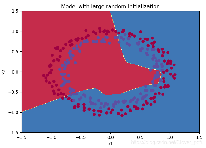
plt.title("Model with large random initialization")
axes = plt.gca()
axes.set_xlim([-1.5, 1.5])
axes.set_ylim([-1.5, 1.5])
init_utils.plot_decision_boundary(lambda x: init_utils.predict_dec(parameters, x.T), train_X, train_Y)

（注：需要把读取并绘制数据的代码中is_plot()改成false，并删除plt.show()）

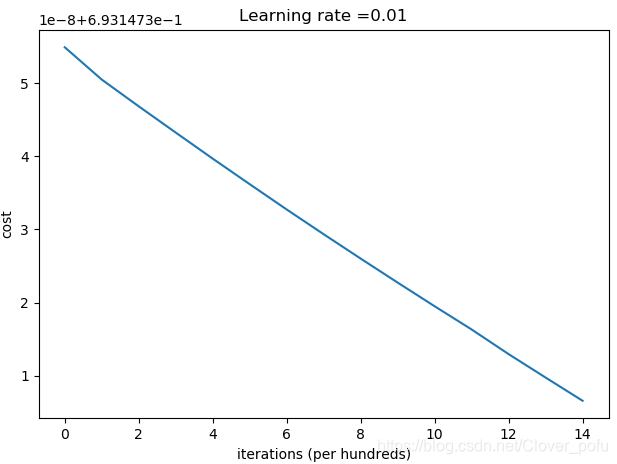
第0次迭代，成本值为：0.6931473549048267
第1000次迭代，成本值为：0.6931473504885134
第2000次迭代，成本值为：0.6931473468317759
第3000次迭代，成本值为：0.6931473432446151
第4000次迭代，成本值为：0.6931473396813665
第5000次迭代，成本值为：0.6931473361903396
第6000次迭代，成本值为：0.6931473327310922
第7000次迭代，成本值为：0.6931473293491259
第8000次迭代，成本值为：0.6931473260187053
第9000次迭代，成本值为：0.6931473227372426
第10000次迭代，成本值为：0.6931473195009528
第11000次迭代，成本值为：0.6931473163278133
第12000次迭代，成本值为：0.693147312959552
第13000次迭代，成本值为：0.6931473097541097
第14000次迭代，成本值为：0.6931473065831708
训练集：
Accuracy: 0.4633333333333333
测试集：
Accuracy: 0.48

从这部分测试可得到以下结论：

• 训练集和测试集准确率都很低。
• 优化速度过慢。
  从model函数的参数表我们可以看到，layers_dims=[X.shape[0],10,5,1]，算是一个深层网络，可能会出现梯度消失或者梯度爆炸的情况。下面尝试用抑制梯度异常的系数初始化W，看看效果如何。

抑制梯度异常初始化

在init_utils.py文件中，找到前向传播函数forward_propagation()，可以看到，用的激活函数是ReLU。在吴恩达的教学视频中提到，为了避免梯度爆炸或梯度消失，针对ReLU激活函数可以在初始化权重时，乘以一个系数： $\sqrt{\frac{2}{上一层的维数}}$

def initialize_parameters_he(layers_dims):
    np.random.seed(3)               # 指定随机种子
    parameters = {}
    L = len(layers_dims)            # 层数
    
    for l in range(1, L):
        parameters['W' + str(l)] = np.random.randn(layers_dims[l], layers_dims[l - 1]) * np.sqrt(2 / layers_dims[l - 1])
        parameters['b' + str(l)] = np.zeros((layers_dims[l], 1))
        
        #使用断言确保我的数据格式是正确的
        assert(parameters["W" + str(l)].shape == (layers_dims[l],layers_dims[l-1]))
        assert(parameters["b" + str(l)].shape == (layers_dims[l],1))
        
    return parameters

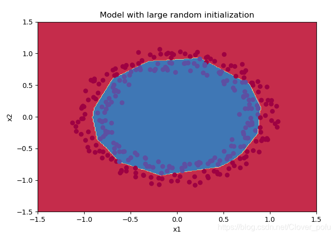
把上面这段代码写到测试并绘制分类结果的代码之前。运行后得到的结果如下：(注：记得调用model函数时，把initialization的参数从“random”改成“he”）

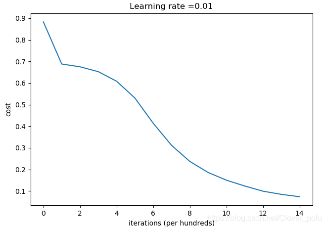
第0次迭代，成本值为：0.8830537463419761
第1000次迭代，成本值为：0.6879825919728063
第2000次迭代，成本值为：0.6751286264523371
第3000次迭代，成本值为：0.6526117768893807
第4000次迭代，成本值为：0.6082958970572938
第5000次迭代，成本值为：0.5304944491717495
第6000次迭代，成本值为：0.4138645817071794
第7000次迭代，成本值为：0.3117803464844441
第8000次迭代，成本值为：0.23696215330322562
第9000次迭代，成本值为：0.18597287209206834
第10000次迭代，成本值为：0.15015556280371806
第11000次迭代，成本值为：0.12325079292273546
第12000次迭代，成本值为：0.09917746546525934
第13000次迭代，成本值为：0.08457055954024278
第14000次迭代，成本值为：0.07357895962677369
训练集：
Accuracy: 0.9933333333333333
测试集：
Accuracy: 0.96

这样做之后分类结果顺眼多了，测试集的准确率也达到了96%。
 

part3——梯度检验

题目陈述

You are part of a team working to make mobile payments available globally, and are asked to build a deep learning model to detect fraud–whenever someone makes a payment, you want to see if the payment might be fraudulent, such as if the user’s account has been taken over by a hacker.
But backpropagation is quite challenging to implement, and sometimes has bugs. Because this is a mission-critical application, your company’s CEO wants to be really certain that your implementation of backpropagation is correct. Your CEO says, “Give me a proof that your backpropagation is actually working!” To give this reassurance, you are going to use “gradient checking”.

您的团队致力于在全球范围内提供移动支付服务，现需要您构建一个深度学习模型来检测欺诈行为——无论何时有人进行支付，您都要查看支付是否是欺诈性的，例如用户的帐户是否已被黑客接管。
但是反向传播在实现上是很有挑战性的，而且有时还有bug，所以您公司的CEO希望确定反向传播的实现是正确的。你的首席执行官说，“给我一个证据，证明你的反向传播确实有效！” 为了保证这一点，你将使用“梯度检查”。

再新建一个.py文件。(提前说明一下，梯度检验这部分写得我真看不出有什么意义，只是照抄了原文，等日后有空了再回来编辑。)

导入库

import numpy as np
import sklearn
import sklearn.datasets
import gc_utils     #第三部分，梯度校验

前向传播函数

def forward_propagation(x,theta):

    J = np.dot(theta,x)
    
    return J

反向传播函数

def backward_propagation(x,theta):
    
    dtheta = x
    
    return dtheta

梯度检验函数

def gradient_check(x,theta,epsilon=1e-7):

    thetaplus = theta + epsilon                               # Step 1
    thetaminus = theta - epsilon                              # Step 2
    J_plus = forward_propagation(x, thetaplus)                # Step 3
    J_minus = forward_propagation(x, thetaminus)              # Step 4
    gradapprox = (J_plus - J_minus) / (2 * epsilon)           # Step 5
    
    
    #检查gradapprox是否足够接近backward_propagation（）的输出
    grad = backward_propagation(x, theta)
    
    numerator = np.linalg.norm(grad - gradapprox)                      # Step 1'
    denominator = np.linalg.norm(grad) + np.linalg.norm(gradapprox)    # Step 2'
    difference = numerator / denominator                               # Step 3'
    
    if difference < 1e-7:
        print("梯度检查：梯度正常!")
    else:
        print("梯度检查：梯度超出阈值!")
    
    return difference

测试

输入以下代码并运行

#测试gradient_check
print("-----------------测试gradient_check-----------------")
x, theta = 2, 4
difference = gradient_check(x, theta)
print("difference = " + str(difference))

得到以下结果：

-----------------测试gradient_check-----------------
梯度检查：梯度正常!
difference = 2.919335883291695e-10