本文结合http://www.cnblogs.com/hapjin/p/6078530.html等众多文章以及Python版本代码来解析逻辑回归并实现
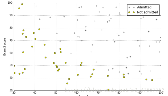
首先问题描述:使用逻辑回归函数根据学生的考试成绩来判断该学生是否可以入学。
训练数据的成绩样例如下:第一列表示第一次考试成绩,第二列表示第二次考试成绩,第三列表示入学结果(0--不能入学,1--可以入学)
34.62365962451697,78.0246928153624,0
30.28671076822607,43.89499752400101,0
35.84740876993872,72.90219802708364,0
60.18259938620976,86.30855209546826,1
......
......1.逻辑回归
1.1数据加载及可视化
首先是加载数据:
import numpy as np
import matplotlib.pyplot as plt
datafile='\ex2data1.txt'
cols=np.loadtxt(datafile,delimiter=',',usecols=(0,1,2),unpack=True)
X=np.transpose(np.array(cols[:-1]))
y=np.transpose(np.array(cols[-1:]))
m=y.size
X=np.insert(X,0,1,axis=1)
# 1.1 Visualizing the data
pos=np.array([X[i] for i in range(X.shape[0]) if y[i]==1])
neg=np.array([X[i] for i in range(X.shape[0]) if y[i]==0])
其中,X 取数据的所有行的第一列和第二列,向量 y 取数据的第三列加载完数据之后,执行以下代码,获取数据中正例的样本(入学),以及反例的样本(不能入学)个数,再用将图形画出来
#Divide the sample into two: ones with positive classification, one with null classification
pos= np.array([X[i]for i inxrange(X.shape[0])if y[i] ==1])
neg= np.array([X[i]for i inxrange(X.shape[0])if y[i] ==0])
#Check to make sure I included all entries
#print "Included everything? ",(len(pos)+len(neg) == X.shape[0])
defplotData():
    plt.figure(figsize=(10,6))
    plt.plot(pos[:,1],pos[:,2],'k+',label='Admitted')
    plt.plot(neg[:,1],neg[:,2],'yo',label='Not admitted')
    plt.xlabel('Exam 1 score')
    plt.ylabel('Exam 2 score')
    plt.legend()
    plt.grid(True)

plotData()
执行的结果如下:
1.2 实现sigmoid函数
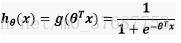
一般来说,回归问题不用在分类问题上,因为回归是连续性模型,而且受噪声影响比较大,如果非要应用到分类问题上,可以使用对数回归。
对数回归本质上是线性回归,只是在特征到结果的映射中加入了一层函数映射,即先把特征线性求和,然后使用函数g(z)作为假设函数来预测,g(z)可以将连续值映射到0和1上。对数回归的假设函数如下,线性回归假设函数只是θx。
实现代码如下:
from scipy.special import expit #Vectorizedsigmoid function

#Hypothesis function and cost function for logistic regression
defh(mytheta,myX):#Logistic hypothesis function
    return expit(np.dot(myX,mytheta))
1.2 模型的代价函数
什么是代价函数呢?把训练好的模型对新数据进行预测,那预测结果有好有坏。因此,就用cost function来衡量预测的"准确性"。cost function越小,表示测的越准。这里的代价函数的本质是”最小二乘法“
代价函数的最原始的定义是下面的这个公式:可见,它是关于theta的函数。(X,y 是已知的,由training set 中的数据确定了)

若直接将sigmoid函数带入到这个式子中,结果是一个非凸函数
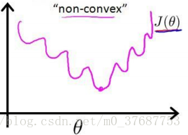
这就意味着,代价函数会有很多局部最小值。所以得换个思路,用概率的角度去求解,由于这是一个二值分类问题,代价函数我们可以用伯努利公式来表示:

既然如此,那么如果能求得代价函数最大时候的θ,即最大似然估计的参数,然后再取反,就能使代价函数最小了,为了计算方便,这里我们取log计算:

代码如下:
def computeCost(mytheta,myX,myy,mylambda=0.):
    """
    theta_start is an n- dimensional vector of initial theta guess
    X is matrix with n- columns and m- rows
    y is a matrix with m- rows and 1 column
    Note this includes regularization, if you set mylambda to nonzero
    For the first part of the homework, the default 0. is used for mylambda
    """
    #note to self: *.shape is (rows, columns)
    term1 = np.dot(-np.array(myy).T,np.log(h(mytheta,myX)))
    term2 = np.dot((1-np.array(myy)).T,np.log(1-h(mytheta,myX)))
    return float( (1./m)* ( np.sum(term1- term2)) )
1.3 梯度下降算法
用梯度下降算法来实现参数θ的不断更新,然后带入到代价函数中不停计算,其公式为:
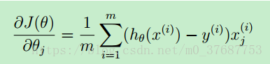
但是在Python中,提供了fmin函数可以直接计算得到最优的参数θ,其代码如下:
def optimizeTheta(mytheta,myX,myy,mylambda=0.):
    result=optimize.fmin(computeCost,x0=mytheta,args=(myX,myy,mylambda),
                         maxiter=400,full_output=True)
    return result[0],result[1]

theta,mincost=optimizeTheta(initial_theta,X,y)

print (computeCost(theta,X,y))
关于optimize.fmin()的函数详细解释,这里是传送门
https://docs.scipy.org/doc/scipy-0.19.1/reference/generated/scipy.optimize.fmin.html
1.4 边界函数的绘制
代码如下:
#Plotting the decision boundary: two points, draw a line between
#Decision boundary occurs when h = 0, or when
#theta0 + theta1*x1 + theta2*x2 = 0
#y=mx+b is replaced by x2 = (-1/thetheta2)(theta0 + theta1*x1)

boundary_xs= np.array([np.min(X[:,1]), np.max(X[:,1])])
boundary_ys= (-1./theta[2])*(theta[0]+ theta[1]*boundary_xs)
plotData()
plt.plot(boundary_xs,boundary_ys,'b-',label='Decision Boundary')
plt.legend()
结果如图:

1.5 模型的评估
以上方法获得最优参数后,现在带入一组数据进行预测,并带入到sigmoid中检测已有的数据的正确率。代码如下:
def makePrediction(mytheta, myx):
    return h(mytheta,myx) >=0.5

#Compute the percentage of samples I got correct:
pos_correct=float(np.sum(makePrediction(theta,pos)))
neg_correct=float(np.sum(np.invert(makePrediction(theta,neg))))
tot=len(pos)+len(neg)
prcnt_correct=float(pos_correct+neg_correct)/tot
print ("Fraction of training samples correctly predicted: %f."% prcnt_correct)

#For a student with an Exam 1 score of 45 and an Exam 2 score of 85,
#you should expect to see an admission probability of 0.776.
print (h(theta,np.array([1,45.,85.])))
2. 正则化逻辑回归
2.1 特征映射
为什么需要特征映射呢?特征映射的好处在于从每个特征中能创造出更多的特征,在这里,我们将特征映射到六次幂,结果如图

这样映射的结果,将两个特征的向量转换为28维响亮,在这个高维向量上训练的回归分类器有更复杂的决策边界,在绘制时会呈现出非线性形状。代码如下:
#This code I took from someone else (the OCTAVE equivalent was provided in the HW)
defmapFeature( x1col, x2col ):
    """
    Function that takes in a column of n- x1's, a column of n- x2s, and builds
    a n- x 28-dim matrix of featuers as described in the homework assignment
    """
    degrees =6
    out = np.ones( (x1col.shape[0],1) )

    for i inrange(1, degrees+1):
        for j inrange(0, i+1):
            term1 = x1col ** (i-j)
            term2 = x2col ** (j)
            term  = (term1 * term2).reshape( term1.shape[0],1 )
            out   = np.hstack(( out, term ))
    return out
2.2 正则化
为什么需要正则化?因为特征映射的过程中生成了太多高次项,当模型的特征(feature variables)非常多,而训练的样本数目(training set)又比较少,会出现过拟合的问题。如果我们发现了过拟合问题,应该如何处理?
1. 丢弃一些不能帮助我们正确预测的特征。可以是手工选择保留哪些特征,或者使用一些模型选择的算法来帮忙(例如 PCA)
2. 正则化。保留所有的特征,但是减少参数的大小(magnitude)
选择正则化,就需要减少高幂次的特征变量的影响,为此我们引入的罚项,假如我们有非常多的特征,我们并不知道其中哪些特征我们要惩罚,我们将对所有的特征进行惩罚。公式如图所示

也可以表示为:

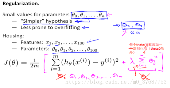
λ为正则化参数,如果选择的正则化参数λ过大,则会把所有的参数都最小化了,导致模型变成hθ(x)=θ0,造成欠拟合。 所以对于正则化,我们要取一个合理的λ的值,这样才能更好的应用正则化。
其代码如下:
#Create feature-mapped X matrix
mappedX= mapFeature(X[:,1],X[:,2])

initial_theta= np.zeros((mappedX.shape[1],1))
computeCost(initial_theta,mappedX,y)

def computeCost(mytheta,myX,myy,mylambda=0.): #注意这里和上面的函数重名了,可自行改变函数名称
    """
    theta_start is an n- dimensional vector of initial theta guess
    X is matrix with n- columns and m- rows
    y is a matrix with m- rows and 1 column
    Note this includes regularization, if you set mylambda to nonzero
    For the first part of the homework, the default 0. is used for mylambda
    """
    #note to self: *.shape is (rows, columns)
    term1 = np.dot(-np.array(myy).T,np.log(h(mytheta,myX)))
    term2 = np.dot((1-np.array(myy)).T,np.log(1-h(mytheta,myX)))
    regterm = (mylambda/2)* np.sum(np.dot(mytheta[1:].T,mytheta[1:]))#Skip theta0
returnfloat( (1./m)* ( np.sum(term1- term2) + regterm ) )注意这里求罚项的时候跳过了θ0,为什么跳过了第一项参数呢,Andrew在其机器学习课程中对此的解释是,按照惯例来讲,不去对θ0进行惩罚,因此 θ0 的值是大的,这就是一个约定,但其实在实践中这只会有非常小的差异,无论你是否包括θ0这项,结果只有非常小的差异。
2.3 最优参数解计算
def optimizeRegularizeTheta(mytheta,myX,myy,mylambda=0.):
    result = optimize.minimize(computeCost, mytheta, args=(myX, myy, mylambda), method='BFGS',
                               options={"maxiter": 500, "disp": False})
    return np.array([result.x]),result.fun

theta,mincost=optimizeRegularizeTheta(initial_theta,mappedX,y)
关于optimize.minimize()函数的解释详见传送门:
https://docs.scipy.org/doc/scipy-0.18.1/reference/generated/scipy.optimize.minimize.html
2.4 绘制边界
defplotBoundary(mytheta, myX, myy, mylambda=0.):
    """
    Function to plot the decision boundary for arbitrary theta, X, y, lambda value
    Inside of this function is feature mapping, and the minimization routine.
    It works by making a grid of x1 ("xvals") and x2 ("yvals") points,
    And for each, computing whether the hypothesis classifies that point as
    True or False. Then, a contour is drawn with a built-in pyplot function.
    """
    theta, mincost = optimizeRegularizedTheta(mytheta,myX,myy,mylambda)
    xvals = np.linspace(-1,1.5,50)
    yvals = np.linspace(-1,1.5,50)
    zvals = np.zeros((len(xvals),len(yvals)))
    for i inrange(len(xvals)):
        for j inrange(len(yvals)):
            myfeaturesij = mapFeature(np.array([xvals[i]]),np.array([yvals[j]]))
            zvals[i][j] = np.dot(theta,myfeaturesij.T)
    zvals = zvals.transpose()

    u, v = np.meshgrid( xvals, yvals )
    mycontour = plt.contour( xvals, yvals, zvals, [0])
    #Kind of a hacky way to display a text on top of the decision boundary
    myfmt = { 0:'Lambda = %d'%mylambda}
    plt.clabel(mycontour, inline=1, fontsize=15, fmt=myfmt)
plt.title("Decision Boundary")注意1:其中linspace函数的参数含义为linspace(start, stop, num=50, endpoint=True, retstep=False, dtype=None)在指定的间隔内返回均匀间隔的数字。
注意2:引用文章https://www.cnblogs.com/happylion/p/4188352.html写的内容,我们在u,v轴上画出一个区域的数据格,把这个区域里面所有的[u,v]通过map_function 得到每一个28维的x向量,然后通过,得到这个区域所有对应的z,然后通过在这些z中画出z=0的等高线,就得到了的这个分界面。
为什么要对z转置?假设区域如图所示

当i=1,v=2的时候,那么z(1,2)就是图中的红点对应的z值,那么循环完之后就是有一个z矩阵,
那么接下来我们用contour这个画等高线,后面的输入是(u,v,z,[0,0]),这里的意思是根据u,v向量给出的坐标,然后和对应的z得到z的曲面,然后后面的[0,0]意思是画出z=0和z=0之间的等高线,也就是画出z=0的等高线。这里有一个地方要注意的是u,v向量给出的坐标,然后和z对应的方式是:比如u的第一个元素和v的第二个元素,对应的是z矩阵的第二行第一列z(2,1),也就是u对应的是矩阵z第几列,v对应的是矩阵z的第几行。然而,我们根据之前循环得到的矩阵知道,那里的z(2,1)是当i=2,v=1得到的,也就是u=2(u的第二个元素),v=1(v的第一个元素),所以我们需要把循环得到的z转置才可以使用contour函数。
最后绘制不同lambda所得到的结果,代码如下:
#Build a figure showing contours for various values of regularization parameter, lambda
#It shows for lambda=0 we are overfitting, and for lambda=100 we are underfitting
plt.figure(figsize=(12,10))
plt.subplot(221)
plotData()
plotBoundary(theta,mappedX,y,0.)

plt.subplot(222)
plotData()
plotBoundary(theta,mappedX,y,1.)

plt.subplot(223)
plotData()
plotBoundary(theta,mappedX,y,10.)

plt.subplot(224)
plotData()
plotBoundary(theta,mappedX,y,100.)
结果如图:

3. 总结
文章是我结合各大网站中关键点以及自己的一些理解后提取出来的内容,感谢文中引用到的链接的优秀文章,代码中之前有很多隐晦不懂的地方,这里也尽力作出了解释,这个是Python版本,但是和Matlab内容差别不大,也可以对比理解。由于个人只是一名初学者,文章中可能存在着一些疏漏,或是一些错误的地方,希望大家谅解,也请大家指正,共同进步。