个人对Kaggle预测房价的探讨,附思路和源代码。
受个人能力限制,存在诸多不足。
仅供参考。欢迎讨论。
目录
1:分析准备
打开train文档,先熟悉数据。

先看看数据,到底什么东西:
import numpy as np
import pandas as pd

data =pd.read_csv(r'./source data/train.csv')
print(data.head())
print("----------------------------------")
print(format(data.shape))
print("----------------------------------")
print(data.info())
结果如下:
<class 'pandas.core.frame.DataFrame'>
RangeIndex: 1460 entries, 0 to 1459
Data columns (total 81 columns):
Id               1460 non-null int64
MSSubClass       1460 non-null int64
MSZoning         1460 non-null object
LotFrontage      1201 non-null float64
LotArea          1460 non-null int64
Street           1460 non-null object
Alley            91 non-null object
LotShape         1460 non-null object
LandContour      1460 non-null object
Utilities        1460 non-null object
LotConfig        1460 non-null object
LandSlope        1460 non-null object
Neighborhood     1460 non-null object
Condition1       1460 non-null object
Condition2       1460 non-null object
BldgType         1460 non-null object
HouseStyle       1460 non-null object
OverallQual      1460 non-null int64
OverallCond      1460 non-null int64
YearBuilt        1460 non-null int64
YearRemodAdd     1460 non-null int64
RoofStyle        1460 non-null object
RoofMatl         1460 non-null object
Exterior1st      1460 non-null object
Exterior2nd      1460 non-null object
MasVnrType       1452 non-null object
MasVnrArea       1452 non-null float64
ExterQual        1460 non-null object
ExterCond        1460 non-null object
Foundation       1460 non-null object
BsmtQual         1423 non-null object
BsmtCond         1423 non-null object
BsmtExposure     1422 non-null object
BsmtFinType1     1423 non-null object
BsmtFinSF1       1460 non-null int64
BsmtFinType2     1422 non-null object
BsmtFinSF2       1460 non-null int64
BsmtUnfSF        1460 non-null int64
TotalBsmtSF      1460 non-null int64
Heating          1460 non-null object
HeatingQC        1460 non-null object
CentralAir       1460 non-null object
Electrical       1459 non-null object
1stFlrSF         1460 non-null int64
2ndFlrSF         1460 non-null int64
LowQualFinSF     1460 non-null int64
GrLivArea        1460 non-null int64
BsmtFullBath     1460 non-null int64
BsmtHalfBath     1460 non-null int64
FullBath         1460 non-null int64
HalfBath         1460 non-null int64
BedroomAbvGr     1460 non-null int64
KitchenAbvGr     1460 non-null int64
KitchenQual      1460 non-null object
TotRmsAbvGrd     1460 non-null int64
Functional       1460 non-null object
Fireplaces       1460 non-null int64
FireplaceQu      770 non-null object
GarageType       1379 non-null object
GarageYrBlt      1379 non-null float64
GarageFinish     1379 non-null object
GarageCars       1460 non-null int64
GarageArea       1460 non-null int64
GarageQual       1379 non-null object
GarageCond       1379 non-null object
PavedDrive       1460 non-null object
WoodDeckSF       1460 non-null int64
OpenPorchSF      1460 non-null int64
EnclosedPorch    1460 non-null int64
3SsnPorch        1460 non-null int64
ScreenPorch      1460 non-null int64
PoolArea         1460 non-null int64
PoolQC           7 non-null object
Fence            281 non-null object
MiscFeature      54 non-null object
MiscVal          1460 non-null int64
MoSold           1460 non-null int64
YrSold           1460 non-null int64
SaleType         1460 non-null object
SaleCondition    1460 non-null object
SalePrice        1460 non-null int64
dtypes: float64(3), int64(35), object(43)
memory usage: 924.0+ KB
None
train的文档中,具有1460个样本,80个属性,而最后需要的结果只有一个:SalePrice,也就是房价。
所以第一件事,就是得进行整合和分析,看这么多属性分别都是什么,中文都是什么意思。
1.1:数据对应中英文转换
| SalePrice | 以美元出售的房产价格。 |
| MSSubClass | 建筑类 |
| MSZoning | 城市总体规划分区 |
| LotFrontage | 连接物业的街道线 |
| LotArea: | Lot size in square feet 方块大小 |
| Street | 道路入口类型 |
| Alley | 巷类型 |
| LotShape | 地产的外形 |
| LandContour | 地产的扁平化 |
| Utilities | 地产的公用事业类型 |
| LotConfig | 地产配置 |
| LandSlope | 地产的坡 |
| Neighborhood | 城市范围内的物理位置 |
| Condition1 | 接近主干道或铁路 |
| Condition2 | 接近主路或铁路 |
| BldgType | 住宅类型 |
| HouseStyle | 居家风格 |
| OverallQual | 整体质量和表面质量 |
| OverallCond | 总体状态额定值 |
| YearBuilt | 原施工日期 |
| YearRemodAdd | 重塑日期 |
| RoofStyle | 屋顶类型 |
| RoofMatl | 屋顶材料 |
| Exterior1st | 房屋外墙 |
| Exterior2nd | 外部第二层:房屋外部覆盖物 |
| MasVnrType | 圬工单板型 |
| MasVnrArea | 砌体单板覆盖面积 |
| ExterQual: | 外观材质 |
| ExterCond | 外墙材料的现状 |
| Foundation | 地基类型 |
| BsmtQual | 地下室的高度 |
| BsmtCond | 地下室概况 |
| BsmtExposure: | 走道或花园式地下室墙 |
| BsmtFinType1 | 地下室竣工面积质量 |
| BsmtFinSF1 | 1型成品面积 |
| BsmtFinType2 | 第二成品区域的质量(如果存在) |
| BsmtFinSF2 | 2型成品面积 |
| BsmtUnfSF | 地下室面积 |
| TotalBsmtSF | 地下室面积总计面积 |
| Heating | 暖气方式 |
| HeatingQC | 暖气质量与条件 |
| CentralAir | 空调 |
| Electrical | 电气系统 |
| 1stFlrSF | 一楼面积 |
| 2ndFlrSF | 二楼面积 |
| LowQualFinSF | 低质量完工面积(所有楼层) |
| GrLivArea | 高档(地面)居住面积 |
| BsmtFullBath | 地下室全浴室 |
| BsmtHalfBath | 地下室半浴室 |
| FullBath | 高档浴室 |
| HalfBath | 半日以上洗澡浴室 |
| Bedroom | 地下室层以上的卧室数 |
| Kitchen | 厨房数量 |
| KitchenQual | 厨房品质 |
| TotRmsAbvGrd | 总房间(不包括浴室) |
| Functional | 家庭功能评级 |
| Fireplaces | 壁炉数 |
| FireplaceQu | 壁炉质量 |
| GarageType | 车库位置 |
| GarageYrBlt | 车库建成年 |
| GarageFinish | 车库的内饰 |
| GarageCars | 车库容量大小 |
| GarageArea | 车库大小 |
| GarageQual | 车库质量 |
| GarageCond | 车库状况 |
| PavedDrive | 铺好的车道 |
| WoodDeckSF | 木制甲板面积 |
| OpenPorchSF | 外部走廊面积 |
| EnclosedPorch | 闭走廊面积 |
| 3SsnPorch: | 三季走廊面积 |
| ScreenPorch | 屏风走廊面积 |
| PoolArea | 泳池面积 |
| PoolQC | 泳池的质量 |
| Fence | 围栏质量 |
| MiscFeature | 其他类别的杂项特征 |
| MiscVal | 杂项价值 |
| MoSold | 月售出 |
| YrSold | 年销售 |
| SaleType | 销售类型 |
| SaleCondition | 销售条件 |
把这些数据整理成Excel表格。发现很多东西看不明白。
1.2:阅读参考资料。
这么多属性,肯定不可能都用,最简单蠢的方法就是人为提取几个特征值,参考我国国情,考虑地段,面积,是否带泳池,材料等,选择十个八个属性直接进行预测。(不可取)
先看看别人是怎么进行的。
琢磨了半天,,,还是老老实实进行一步一步分析
2:数据分析
先看看需要预测的房价有什么特点,
''
train_data = pd.read_csv(r'./source data/train.csv')
test_data = pd.read_csv(r'./source data/test.csv')
#略过基本信息阶段

#ID这一栏基本没用,干扰信息,考虑是不是删了
train_ID = train_data['Id']
test_ID = test_data['Id']
#train_data.drop("Id", axis= 1, inplace= True)

#研究分析房价数据分布
print(train_data['SalePrice'].describe())
sns.set_style("whitegrid")
sns.distplot(train_data['SalePrice'])
结果如下:
count      1460.000000
mean     180921.195890
std       79442.502883
min       34900.000000
25%      129975.000000
50%      163000.000000
75%      214000.000000
max      755000.000000
Name: SalePrice, dtype: float64
可以看到,房价的平均值大概分布的段位,以及最高的房子,估计是别墅,也很贵。
没研究出什么关系。
| GrLivArea | 高档(地面)居住面积 |
接下来看看这个,这个居住面积和房价肯定有关系吧,
#居住面积和房价
fig, ax =plt.subplots()
ax.scatter( x  = train_data['GrLivArea'], y = train_data['SalePrice'])
plt.ylabel('SalePrice')
plt.xlabel('GrLivArea')
plt.show()
结果如下
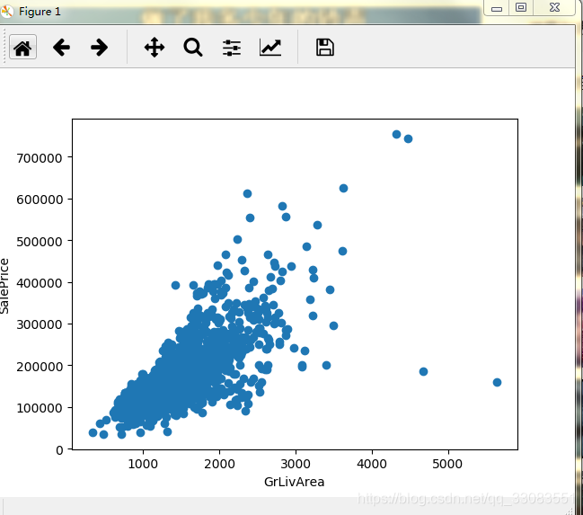
对应的面积越小,房价越便宜,符合我们日常的常识。
奇异点也比较少,完全可以解释,这部分数据看起来没问题。
同理,总房间数和房价应该也是正比。

其实到这会,我们可以看到,右边这个点,我完全可以把他当做干扰数据pass掉,,但是先保存着,
除此之外,新房应该比旧房子贵,这个没异议吧?我们看看数据。
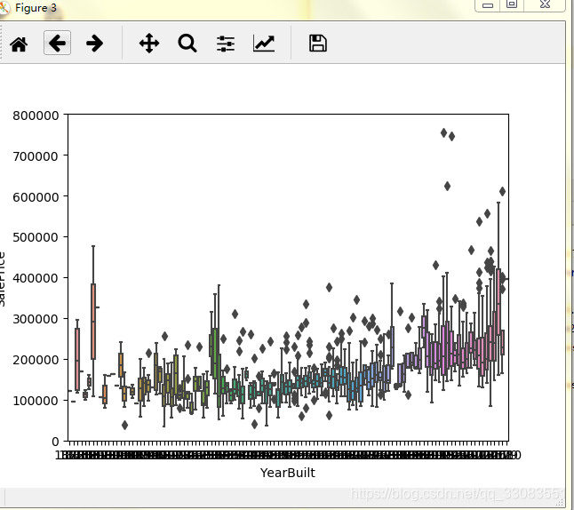
emmm...大概是没问题的。
看下热力图:
corrmat = train_data.corr()
f, ax =plt.subplots()
sns.heatmap(corrmat, vmax=.8, square= True)

k=10
cols = corrmat.nlargest(k,'SalePrice')['SalePrice'].index
cm = np.corrcoef(train_data[cols].values.T)
sns.set(font_scale=1.25)
hm = sns.heatmap(cm, cbar=True, annot=True, square=True, fmt='.2f', annot_kws={'size': 10}, yticklabels=cols.values, xticklabels=cols.values)
plt.show()
排名前三的有:住房质量,高档地面居住面积,车库容量大小。
感觉车库国人不在乎,国外的人人有车,那么问题来了。我什么时候买车????
还有一些变量之间有很强的相关性, 这意思要么2选一,要么线性组合--------这是一个思路
(就是可以降维,用A来表示B:B=0.82A+0.02)
删除多余数据
这有几个奇异点,不知道怎么处理,简单点,切了吧。
fig, ax = plt.subplots()
ax.scatter(x = train_data['GrLivArea'], y = train_data['SalePrice'])
plt.ylabel('SalePrice', fontsize=13)
plt.xlabel('GrLivArea', fontsize=13)
plt.show()

#挑除异常点
train_data = train_data.drop(train_data[train_data['GrLivArea']>4000].index)
fig, ax = plt.subplots()
ax.scatter(train_data['GrLivArea'], train_data['SalePrice'])
plt.ylabel('SalePrice')
plt.xlabel('GrLivArea')
plt.show()
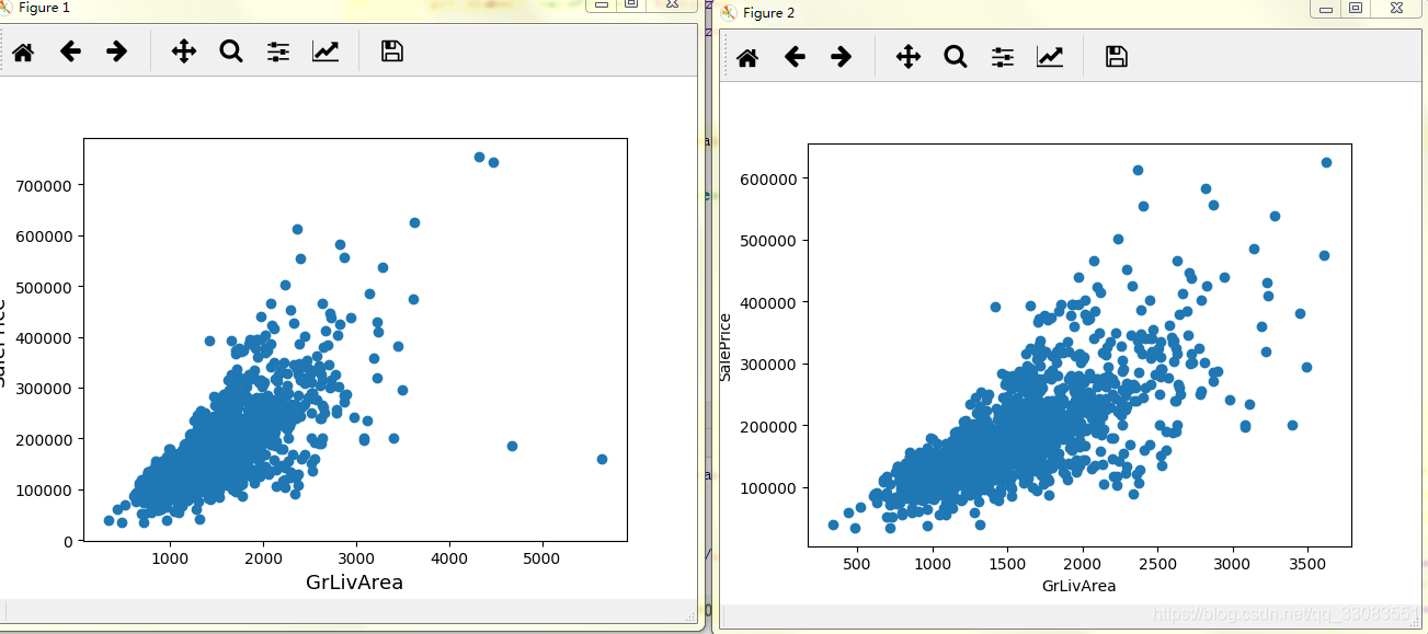
其实我想把价格大于60万的也切了,会更整洁,后来思考下有点过分,那算了吧。
房价的数据不平滑,我们需要把离散的数据拟合成连续的平滑的数据。
用常用的log(x+1)
#让数据更加平滑
#log1p就是log(1+x)
train_data['SalePrice'] = np.log1p(train_data['SalePrice'])
sns.distplot(train_data['SalePrice'] )
确实平滑了,但是直接这样处理太过于粗糙。
看看还能做什么
1:拟合一下,需要导入两个库
from scipy import stats
from scipy.stats import norm,skew

#让数据更加平滑
#log1p就是log(1+x)
train_data['SalePrice'] = np.log1p(train_data['SalePrice'])
sns.distplot(train_data['SalePrice'] )

#看一下函数拟合
(mu, sigma) = norm.fit(train_data['SalePrice'])
print('\n mu ={:.2f} and sigma = {:.2f} \n' .format(mu,sigma))

#画个图,看下分布
plt.legend(['Normal dist. ($\mu=$ {:.2f} and $\sigma=$ {:.2f} )'.format(mu, sigma)],
            loc='best')
plt.ylabel('Frequency')
plt.title('SalePrice distribution')
#再话个QQ分布,不知道为啥,老外特别喜欢这个,
fig = plt.figure()
res = stats.probplot(train_data['SalePrice'], plot=plt)
plt.show()
结果为
mu =12.02 and sigma = 0.40

做到这一步可以开始初步的尝试了。
3:初步尝试
国际惯例,先把测试集和训练集结合在一起
#开始初步的尝试
#1.通用步骤,把test和train联合在一起。
train_data = train_data.drop(train_data[train_data['GrLivArea']>4000].index)
train= train_data.shape[0]
test = test_data.shape[0]
y_train = train_data.SalePrice.values
all_data = pd.concat((train_data, test_data)).reset_index(drop=True,)

all_data.drop(['SalePrice'], axis =1, inplace = True)
然后开始处理缺失数据,
有3种处理方式:
1:默认如果没有车库之类的,就没有车,这种硬相关的东西
2: 如果缺失值较少的,用众数弥补。
3:数据里面 比如地下室之类的,为Nan,说明没有地下室,把面积用0来填充,
符合常理(在提高里面就可以写,数据收到主观因素干扰,可以提升点。。。)
#用None补充的数据
all_data["PoolQC"] = all_data["PoolQC"].fillna("None")
all_data["MiscFeature"] = all_data["MiscFeature"].fillna("None")
all_data["Alley"] = all_data["Alley"].fillna("None")
all_data["Fence"] = all_data["Fence"].fillna("None")
all_data["FireplaceQu"] = all_data["FireplaceQu"].fillna("None")
#LotFrontage这个属性,假定为同一个街道的属性相似。

all_data["LotFrontage"] = all_data.groupby("Neighborhood")["LotFrontage"].transform(
    lambda x: x.fillna(x.median()))
#  'GarageType', 'GarageFinish', 'GarageQual' and 'GarageCond' 这几个属性的空缺,十有八九是没有
for col in ('GarageType', 'GarageFinish', 'GarageQual', 'GarageCond'):
    all_data[col] = all_data[col].fillna('None')
#有一些硬件,没有就是零,然后同一个街道默认为一样
#同时,假定没有车库就没车,(确实不合理,但是好统计)
for col in ('GarageYrBlt', 'GarageArea', 'GarageCars'):
    all_data[col] = all_data[col].fillna(0)

#'BsmtFinSF1', 'BsmtFinSF2', 'BsmtUnfSF','TotalBsmtSF', 'BsmtFullBath', 'BsmtHalfBath' 这些没有代表面积为0
for col in ('BsmtFinSF1', 'BsmtFinSF2', 'BsmtUnfSF','TotalBsmtSF', 'BsmtFullBath', 'BsmtHalfBath'):
    all_data[col] = all_data[col].fillna(0)

for col in ('BsmtQual', 'BsmtCond', 'BsmtExposure', 'BsmtFinType1', 'BsmtFinType2'):
    all_data[col] = all_data[col].fillna('None')

all_data["MasVnrType"] = all_data["MasVnrType"].fillna("None")
all_data["MasVnrArea"] = all_data["MasVnrArea"].fillna(0)
all_data['MSZoning'] = all_data['MSZoning'].fillna(all_data['MSZoning'].mode()[0])

#Utilities这个属性对数据的影响不大,可以将剔除出去
all_data = all_data.drop(['Utilities'], axis=1)
all_data["Functional"] = all_data["Functional"].fillna("Typ")
#接下来的数据里面,缺失值比较少,用众数来弥补
all_data['Electrical'] = all_data['Electrical'].fillna(all_data['Electrical'].mode()[0])
all_data['KitchenQual'] = all_data['KitchenQual'].fillna(all_data['KitchenQual'].mode()[0])
all_data['Exterior1st'] = all_data['Exterior1st'].fillna(all_data['Exterior1st'].mode()[0])
all_data['Exterior2nd'] = all_data['Exterior2nd'].fillna(all_data['Exterior2nd'].mode()[0])
all_data['SaleType'] = all_data['SaleType'].fillna(all_data['SaleType'].mode()[0])

all_data['MSSubClass'] = all_data['MSSubClass'].fillna("None")
4. 建模
这里直接使用sklearn库。
需要导入几个相关库文件
from sklearn.ensemble import RandomForestRegressor,GradientBoostingRegressor
import xgboost as xgb
import lightgbm as lgb
from sklearn.model_selection import KFold, cross_val_score, train_test_split
from sklearn.metrics import mean_squared_error
然后个人习惯,10次交叉验证:
#10次交叉
n_folds = 10

def rmsle_cv(model):
    kf = KFold(n_folds, shuffle=True, random_state=42).get_n_splits(train.values)
    rmse= np.sqrt(-cross_val_score(model, train.values, y_train, scoring="neg_mean_squared_error", cv = kf))
    return(rmse)
接下来就是直接使用自带的
rfc=RandomForestRegressor(n_estimators=1000)GBoost = GradientBoostingRegressor(n_estimators=3000, learning_rate=0.05,
max_depth=4, max_features='sqrt',
min_samples_leaf=15, min_samples_split=10,
loss='huber', random_state =5)model_xgb = xgb.XGBRegressor(colsample_bytree=0.4603, gamma=0.0468,
learning_rate=0.05, max_depth=3,
min_child_weight=1.7817, n_estimators=2200,
reg_alpha=0.4640, reg_lambda=0.8571,
subsample=0.5213, silent=1,
random_state =7, nthread = -1)model_lgb = lgb.LGBMRegressor(objective='regression',num_leaves=5,
learning_rate=0.05, n_estimators=720,
max_bin = 55, bagging_fraction = 0.8,
bagging_freq = 5, feature_fraction = 0.2319,
feature_fraction_seed=9, bagging_seed=9,
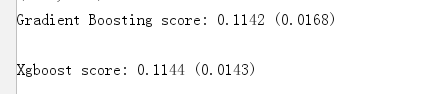
min_data_in_leaf =6, min_sum_hessian_in_leaf = 11)预测:
GBoost.fit(train,y_train)
GBoost_train_pred = GBoost.predict(train)
GB_pred = np.expm1(GBoost.predict(test.values))
预测的结果
![]()
生成提交文件:
sub = pd.DataFrame()
sub['Id'] = test_ID
sub['SalePrice'] = GB_pred
sub.to_csv('submission.csv',index=False)
上传结果

5. git传送门
https://github.com/PANBOHE/HousePrices
-----------------暂时到这告一段落------------
后续继续更新优化。
HPV01-11012019:陆陆续续换了4天整理出来,马马虎虎将就看吧
欢迎关注:

参考文献
【1】周志华,西瓜书(懂的人自然懂)
【2】廖雪峰老师的python教程
【3】Kaggle--房价预测
https://blog.csdn.net/d_i_k_y/article/details/80954546#%E4%B8%80%E8%AE%A4%E8%AF%86%E6%95%B0%E6%8D%AE
【4】Beginner Approach with XGBoost , LightGBM and EDA
https://www.kaggle.com/nephalem98/beginner-approach-with-xgboost-lightgbm-and-eda