房价预测(kaggle调试笔记）

项目描述：

赛题给我们79个描述房屋的特征，要求我们据此预测房屋的最终售价，即对于测试集中每个房屋的ID给出对于的SalePrice字段的预测值，主要考察我们数据清洗、特征工程、模型搭建及调优等方面的技巧。本赛题是典型的回归类问题，评估指标选用的是均方根误差（RMSE），为了使得价格的高低对结果的评估有均等的影响，赛题均方根误差基于预测值和实际值分别取对数对数来计算。
特征初步分析：
1. SalePrice 房屋售价，我们要预测的label，类型：数值型，单位：美元
2. MSSubClass: 建筑的等级，类型：类别型
MSZoning: 区域分类，类型：类别型
LotFrontage: 距离街道的直线距离，类型：数值型，单位：英尺
LotArea: 地皮面积，类型：数值型，单位：平方英尺
Street: 街道类型，类型：类别型
Alley: 巷子类型，类型：类别型
LotShape: 房子整体形状，类型：类别型
LandContour: 平整度级别，类型：类别型
Utilities: 公共设施类型，类型：类别型
LotConfig: 房屋配置，类型：类别型
LandSlope: 倾斜度，类型：类别型
Neighborhood: 市区物理位置，类型：类别型
Condition1: 主干道或者铁路便利程度，类型：类别型
Condition2: 主干道或者铁路便利程度，类型：类别型
BldgType: 住宅类型，类型：类别型
HouseStyle: 住宅风格，类型：类别型
OverallQual: 整体材料和饰面质量，类型：数值型
OverallCond: 总体状况评价，类型：数值型
YearBuilt: 建筑年份，类型：数值型
YearRemodAdd: 改建年份，类型：数值型
RoofStyle: 屋顶类型，类型：类别型
RoofMatl: 屋顶材料，类型：类别型
Exterior1st: 住宅外墙，类型：类别型
Exterior2nd: 住宅外墙，类型：类别型
MasVnrType: 砌体饰面类型，类型：类别型
MasVnrArea: 砌体饰面面积，类型：数值型，单位：平方英尺
ExterQual: 外部材料质量，类型：类别型
ExterCond: 外部材料的现状，类型：类别型
Foundation: 地基类型，类型：类别型
BsmtQual: 地下室高度，类型：类别型
BsmtCond: 地下室概况，类型：类别型
BsmtExposure: 花园地下室墙，类型：类别型
BsmtFinType1: 地下室装饰质量，类型：类别型
BsmtFinSF1: 地下室装饰面积，类型：类别型
BsmtFinType2: 地下室装饰质量，类型：类别型
BsmtFinSF2: 地下室装饰面积，类型：类别型
BsmtUnfSF: 未装饰的地下室面积，类型：数值型，单位：平方英尺
TotalBsmtSF: 地下室总面积，类型：数值型，单位：平方英尺
Heating: 供暖类型，类型：类别型
HeatingQC: 供暖质量和条件，类型：类别型
CentralAir: 中央空调状况，类型：类别型
Electrical: 电力系统，类型：类别型
1stFlrSF: 首层面积，类型：数值型，单位：平方英尺
2ndFlrSF: 二层面积，类型：数值型，单位：平方英尺
LowQualFinSF: 低质装饰面积，类型：数值型，单位：平方英尺
GrLivArea: 地面以上居住面积，类型：数值型，单位：平方英尺
BsmtFullBath: 地下室全浴室，类型：数值
BsmtHalfBath: 地下室半浴室，类型：数值
FullBath: 高档全浴室，类型：数值
HalfBath: 高档半浴室，类型：数值
BedroomAbvGr: 地下室以上的卧室数量，类型：数值
KitchenAbvGr: 厨房数量，类型：数值
KitchenQual: 厨房质量，类型：类别型
TotRmsAbvGrd: 地上除卧室以外的房间数，类型：数值
Functional: 房屋功用性评级，类型：类别型
Fireplaces: 壁炉数量，类型：数值
FireplaceQu: 壁炉质量，类型：类别型
GarageType: 车库位置，类型：类别型
GarageYrBlt: 车库建造年份，类别：数值型
GarageFinish: 车库内饰，类型：类别型
GarageCars: 车库车容量大小，类别：数值型
GarageArea: 车库面积，类别：数值型，单位：平方英尺
GarageQual: 车库质量，类型：类别型
GarageCond: 车库条件，类型：类别型
PavedDrive: 铺的车道情况，类型：类别型
WoodDeckSF: 木地板面积，类型：数值型，单位：平方英尺
OpenPorchSF: 开放式门廊区面积，类型：数值型，单位：平方英尺
EnclosedPorch: 封闭式门廊区面积，类型：数值型，单位：平方英尺
3SsnPorch: 三个季节门廊面积，类型：数值型，单位：平方英尺
ScreenPorch: 纱门门廊面积，类型：数值型，单位：平方英尺
PoolArea: 泳池面积，类型：数值型，单位：平方英尺
PoolQC:泳池质量，类型：类别型
Fence: 围墙质量，类型：类别型
MiscFeature: 其他特征，类型：类别型
MiscVal: 其他杂项特征值，类型：类别型
MoSold: 卖出月份，类别：数值型
YrSold: 卖出年份，类别：数值型
SaleType: 交易类型，类型：类别型
SaleCondition: 交易条件，类型：类别型

kaggle地址：

完整代码地址：

代码梳理：

 一.特征工程

      1. 特征类型分析：数值型特征和类别型特征各有多少。

      2.对数值型特征和类别行特征分别进行特征处理。

       2.1数值型特征：

           1.通过绘制各个特征与Y值（房价）的关系，确认离群点，并去除离群点.

#删除离群点
train = train.drop(train[(train['GrLivArea']>4000) & (train['SalePrice']<300000)].index)

           2.目标值处理： 分析Y值得分布，线性的模型需要正态分布的目标值才能发挥最大的作用。使用probplot函数，绘制正态概率图

            通过分析正太概率图，发现：此时的正态分布属于右偏态分布，即整体峰值向左偏离，并且偏度(skewness)较大，需要对目标值做log转换，以恢复目标值的正态性。

sns.distplot(train['SalePrice'] , fit=norm)
# Get the fitted parameters used by the function
(mu, sigma) = norm.fit(train['SalePrice'])
print( '\n mu = {:.2f} and sigma = {:.2f}\n'.format(mu, sigma))

#Now plot the distribution
plt.legend(['Normal dist. ($\mu=$ {:.2f} and $\sigma=$ {:.2f} )'.format(mu, sigma)],
            loc='best')
plt.ylabel('Frequency')
plt.title('SalePrice distribution')

#Get also the QQ-plot
fig = plt.figure()
res = stats.probplot(train['SalePrice'], plot=plt)
plt.show()

mu = 180932.92 and sigma = 79467.79

        

         3.将训练数据和测试数据合并，一起进行特征工程。

         4.分析数据确实情况：缺失数据可视化

all_data_na = (all_data.isnull().sum() / len(all_data)) * 100
all_data_na = all_data_na.drop(all_data_na[all_data_na == 0].index).sort_values(ascending=False)[:30]
missing_data = pd.DataFrame({'Missing Ratio' :all_data_na})

f, ax = plt.subplots(figsize=(15, 12))
plt.xticks(rotation='90')
sns.barplot(x=all_data_na.index, y=all_data_na)
plt.xlabel('Features', fontsize=15)
plt.ylabel('Percent of missing values', fontsize=15)
plt.title('Percent missing data by feature', fontsize=15)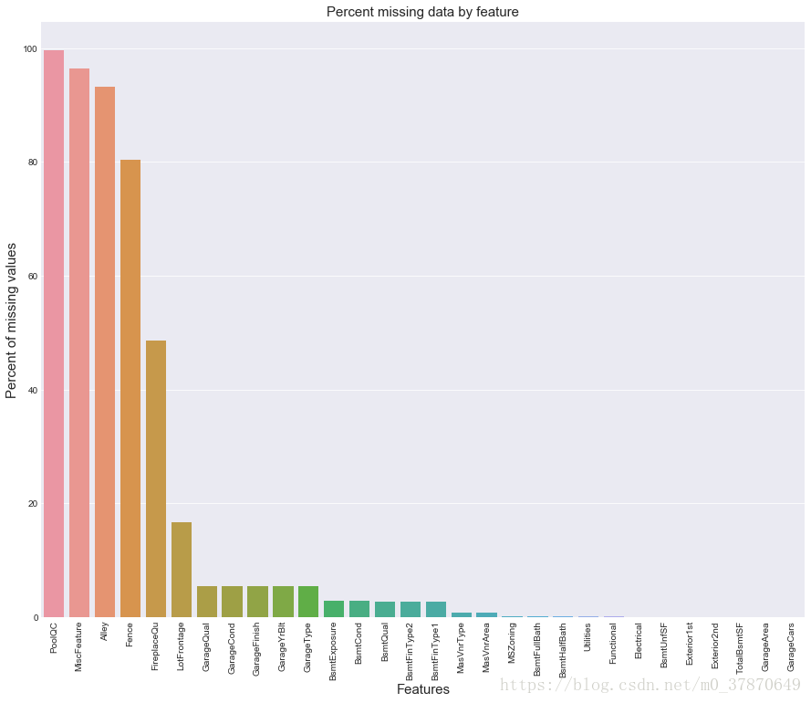

ext(0.5,1,'Percent missing data by feature')

   5 缺失数据处理：确实数据比较多，需要尽心缺失数据处理。

      分析各个特征以及房价的相关性，相关性的分析最好使用热力图

#Correlation map to see how features are correlated with SalePrice
corrmat = train.corr()
plt.subplots(figsize=(12,9))
sns.heatmap(corrmat, vmax=0.9, square=True)

<matplotlib.axes._subplots.AxesSubplot at 0x9cd6e3d358>

  可以看到对角线有一条白线，这代表相同的特征相关性为最高，但值得注意的是，有两个正方形小块：TotaLBsmtSF和1stFlrSF、GarageAreas和GarageCars处。这代表全部建筑面积TotaLBsmtSF与一层建筑面积1stFlrSF成强正相关，车库区域GarageAreas和车库车辆GarageCars成强正相关，那么在填补缺失值的时候就有了依据，我们可以直接删掉一个多余的特征或者使用一个填补另一个。

    7 填补缺失值

       根据上图相关性，以及各个特征的实际含义进行缺失值填充。

all_data["PoolQC"] = all_data["PoolQC"].fillna("None")
all_data["MiscFeature"] = all_data["MiscFeature"].fillna("None")
all_data["Alley"] = all_data["Alley"].fillna("None")
all_data["Fence"] = all_data["Fence"].fillna("None")
all_data["FireplaceQu"] = all_data["FireplaceQu"].fillna("None")
#print(type(all_data.groupby("Neighborhood")["LotFrontage"]))
#print(all_data.groupby("Neighborhood")["LotFrontage"])
#help(all_data.groupby("Neighborhood")["LotFrontage"].transform)

#Group by neighborhood and fill in missing value by the median LotFrontage of all the neighborhood
all_data["LotFrontage"] = all_data.groupby("Neighborhood")["LotFrontage"].transform(
    lambda x: x.fillna(x.median()))

for col in ('GarageType', 'GarageFinish', 'GarageQual', 'GarageCond'):
    all_data[col] = all_data[col].fillna('None')
    
for col in ('GarageYrBlt', 'GarageArea', 'GarageCars'):
    all_data[col] = all_data[col].fillna(0)
    
for col in ('BsmtFinSF1', 'BsmtFinSF2', 'BsmtUnfSF','TotalBsmtSF', 'BsmtFullBath', 'BsmtHalfBath'):
    all_data[col] = all_data[col].fillna(0)
    
for col in ('BsmtQual', 'BsmtCond', 'BsmtExposure', 'BsmtFinType1', 'BsmtFinType2'):
    all_data[col] = all_data[col].fillna('None')
    
all_data["MasVnrType"] = all_data["MasVnrType"].fillna("None")
all_data["MasVnrArea"] = all_data["MasVnrArea"].fillna(0)

all_data['MSZoning'] = all_data['MSZoning'].fillna(all_data['MSZoning'].mode()[0])

#对于'Utilities'这个特征，所有记录均为“AllPub”，除了一个“NoSeWa”和2个NA。 由于拥有'NoSewa'的房子在训练集中，
#因此此特征对预测建模无助。 然后我们可以安全地删除它。
all_data = all_data.drop(['Utilities'], axis=1)

all_data["Functional"] = all_data["Functional"].fillna("Typ")
all_data['Electrical'] = all_data['Electrical'].fillna(all_data['Electrical'].mode()[0])
all_data['KitchenQual'] = all_data['KitchenQual'].fillna(all_data['KitchenQual'].mode()[0])
all_data['Exterior1st'] = all_data['Exterior1st'].fillna(all_data['Exterior1st'].mode()[0])
all_data['Exterior2nd'] = all_data['Exterior2nd'].fillna(all_data['Exterior2nd'].mode()[0])
all_data['SaleType'] = all_data['SaleType'].fillna(all_data['SaleType'].mode()[0])
all_data['MSSubClass'] = all_data['MSSubClass'].fillna("None")
all_data_na = (all_data.isnull().sum() / len(all_data)) * 100
all_data_na = all_data_na.drop(all_data_na[all_data_na == 0].index).sort_values(ascending=False)
missing_data = pd.DataFrame({'Missing Ratio' :all_data_na})
missing_data.head()

8.添加新特征

接下来添加一个重要的特征，因为我们实际在购买房子的时候会考虑总面积的大小，但是此数据集中并没有包含此数据。总面积等于地下室面积+1层面积+2层面积

# Adding total sqfootage feature 
all_data['TotalSF'] = all_data['TotalBsmtSF'] + all_data['1stFlrSF'] + all_data['2ndFlrSF']

9.数据类型转换

9.1 文本类型特征处理 

有些数据实际含义是类别型特征，在此处用了数值表示，需要将其转化为类别型特征

#MSSubClass=The building class
all_data['MSSubClass'] = all_data['MSSubClass'].apply(str)

#Changing OverallCond into a categorical variable
all_data['OverallCond'] = all_data['OverallCond'].astype(str)

接下来 LabelEncoder，对文本类别的特征进行编号。

from sklearn.preprocessing import LabelEncoder
cols = ('FireplaceQu', 'BsmtQual', 'BsmtCond', 'GarageQual', 'GarageCond', 
        'ExterQual', 'ExterCond','HeatingQC', 'PoolQC', 'KitchenQual', 'BsmtFinType1', 
        'BsmtFinType2', 'Functional', 'Fence', 'BsmtExposure', 'GarageFinish', 'LandSlope',
        'LotShape', 'PavedDrive', 'Street', 'Alley', 'CentralAir', 'MSSubClass', 'OverallCond', 
        'YrSold', 'MoSold')
# process columns, apply LabelEncoder to categorical features
for c in cols:
    lbl = LabelEncoder() 
    lbl.fit(list(all_data[c].values))
    all_data[c] = lbl.transform(list(all_data[c].values))

# shape        
print('Shape all_data: {}'.format(all_data.shape))

将类别特征进行哑变量转化（注：此处进行哑变量转化，应该不需要如上进行LabelEncoder？）

all_data = pd.get_dummies(all_data)
print(all_data.shape)

9.2 数值类型特征处理

  对每一个特征的分布进行分析：我们对房价进行分析，不符合正态分布的我们已经将其log转换，使其符合正态分布。那么偏离正态分布的特征我们也对它进行转化

采用偏度分析特征的分布

numeric_feats = all_data.dtypes[all_data.dtypes != "object"].index

# Check the skew of all numerical features
skewed_feats = all_data[numeric_feats].apply(lambda x: skew(x.dropna())).sort_values(ascending=False)
print("\nSkew in numerical features: \n")
skewness = pd.DataFrame({'Skew' :skewed_feats})
skewness.head()

Skew in numerical features: 

Out[16]:

	Skew
MiscVal	21.940
PoolArea	17.689
LotArea	13.109
LowQualFinSF	12.085
3SsnPorch	11.372

采用boxcoxlp将符合正在分布的特征，进行处理，使其符合正态分布。

skewness = skewness[abs(skewness) > 0.75]
print("There are {} skewed numerical features to Box Cox transform".format(skewness.shape[0]))

from scipy.special import boxcox1p
skewed_features = skewness.index
lam = 0.15
for feat in skewed_features:
    #all_data[feat] += 1
    all_data[feat] = boxcox1p(all_data[feat], lam)

10 至此，特征工程出来完毕。

 将数据重分为训练集和测试集

train = all_data[:ntrain]
test = all_data[ntrain:]

------------------------------------------------------------------------------------------

transform使用：

相关参考：Pandas分组运算（groupby）修炼：https://www.cnblogs.com/lemonbit/p/6810972.html

1.调试笔记：

#Group by neighborhood and fill in missing value by the median LotFrontage of all the neighborhood
all_data["LotFrontage"] = all_data.groupby("Neighborhood")["LotFrontage"].transform(
    lambda x: x.fillna(x.median()))

知识点1

print(type(all_data.groupby("Neighborhood")["LotFrontage"]))
print(all_data.groupby("Neighborhood")["LotFrontage"])
help(all_data.groupby("Neighborhood")["LotFrontage"].transform)

打印如下：

<class 'pandas.core.groupby.SeriesGroupBy'>
<pandas.core.groupby.SeriesGroupBy object at 0x0000009CDABC6630>
Help on method transform in module pandas.core.groupby:

transform(func, *args, **kwargs) method of pandas.core.groupby.SeriesGroupBy instance
    Call function producing a like-indexed Series on each group and
    return a Series having the same indexes as the original object
    filled with the transformed values
    
    Parameters
    ----------
    f : function
        Function to apply to each group
    
    Notes
    -----
    Each group is endowed the attribute 'name' in case you need to know
    which group you are working on.
    
    The current implementation imposes three requirements on f:
    
    * f must return a value that either has the same shape as the input
      subframe or can be broadcast to the shape of the input subframe.
      For example, f returns a scalar it will be broadcast to have the
      same shape as the input subframe.
    * if this is a DataFrame, f must support application column-by-column
      in the subframe. If f also supports application to the entire subframe,
      then a fast path is used starting from the second chunk.
    * f must not mutate groups. Mutation is not supported and may
      produce unexpected results.
    
    Returns
    -------
    Series
    
    See also
    --------
    aggregate, transform
    
    Examples
    --------
    
    # Same shape
    >>> df = pd.DataFrame({'A' : ['foo', 'bar', 'foo', 'bar',
    ...                           'foo', 'bar'],
    ...                    'B' : ['one', 'one', 'two', 'three',
    ...                          'two', 'two'],
    ...                    'C' : [1, 5, 5, 2, 5, 5],
    ...                    'D' : [2.0, 5., 8., 1., 2., 9.]})
    >>> grouped = df.groupby('A')
    >>> grouped.transform(lambda x: (x - x.mean()) / x.std())
              C         D
    0 -1.154701 -0.577350
    1  0.577350  0.000000
    2  0.577350  1.154701
    3 -1.154701 -1.000000
    4  0.577350 -0.577350
    5  0.577350  1.000000
    
    # Broadcastable
    >>> grouped.transform(lambda x: x.max() - x.min())
       C    D
    0  4  6.0
    1  3  8.0
    2  4  6.0
    3  3  8.0
    4  4  6.0
    5  3  8.0