ML Lecture 1: Regression - Demo

ML Lecture 1: Regression - Demo

• Youtube
• Bilibili

---

Gradient Descent Demo

用Python实现梯度下降法求解最优参数$w$和$b$。沿用上一节的第一个线性模型：

$$y = b + w x_{cp}$$ 其中， $x_{cp}$是进化前的CP值， $y$是进化后的CP值，参数 $w$是权重（weight），参数 $b$是偏置（bias）。

定义损失函数：

$$L(f) = L(w, b) = \sum_{n=1}^{10} ( \hat{y}^n - (b + wx_{cp}^n) )^2$$
其中， $\hat{y}^n$是第 $n$只pokemon进化后的 真实CP值， $(b + wx_{cp}^n)$是第 $n$只pokemon进化后的模型 预测CP值。

令损失函数$L$分别对参数$w$、$b$求偏导：

$$\frac{\partial L}{\partial w} = \sum_{n=1}^{10} 2( \hat{y}^n - (b + wx_{cp}^n) ) (-x_{cp}^n)$$ $$\frac{\partial L}{\partial b} = \sum_{n=1}^{10} 2( \hat{y}^n - (b + wx_{cp}^n) ) (-1)$$

则梯度下降法的求解过程如下：

1. 选取参数初始值$w_0$、$b_0$，设定一个学习率$lr$
2. 参数迭代更新的公式为： $$w_1 = w_0 - lr \cdot \frac{\partial L}{\partial w}|_{w = w_0, b = b_0}，b_1 = b_0 - lr \cdot \frac{\partial L}{\partial b}|_{w = w_0, b = b_0}$$ $$w_2 = w_1 - lr \cdot \frac{\partial L}{\partial w}|_{w = w_1, b = b_1}，b_2 = b_1 - lr \cdot \frac{\partial L}{\partial b}|_{w = w_1, b = b_1}$$ $$......$$

用Python代码实现如下：

import numpy as np
import matplotlib.pyplot as plt


# 输入10只pokemon进化前的CP值x_data和进化后的CP值y_data
x_data = [338, 333, 328, 207, 226, 25, 179, 60, 208, 606]
y_data = [640, 633, 619, 393, 428, 27, 193, 66, 226, 1591]
# 模型为y_data = b + w * x_data
# 事实上参数w和b有闭式解（Closed Form Solution），有更简洁的求解方法
# 这里主要是为了练习使用梯度下降法


x = np.arange(-200, -100)                    # x是横坐标（参数b）的范围
y = np.arange(-5, 5, 0.1)                    # y是纵坐标（参数w）的范围
Z = np.zeros((len(x), len(y)))               # Z是填充0值的array，有len(x)行，有len(y)列
X, Y = np.meshgrid(x, y)                     # 生成二维空间的网格矩阵，X、Y均是有len(y)行、len(x)列的array
for i in range(len(x)):                      
    for j in range(len(y)):
        b = x[i]                             # 参数b从向量x中取值
        w = y[j]                             # 参数w从向量y中取值
        Z[j][i] = 0                          # 平方损失值的初始值为0
        for n in range(len(x_data)):         # 每一个样本的平方损失值累加，共n个样本
            Z[j][i] += (y_data[n] - b - w * x_data[n]) ** 2
        Z[j][i] = Z[j][i] / len(x_data)      # 总平方损失值/n 


# 设置初始参数
b = -120                                     # 参数b的初始值
w = -4                                       # 参数w的初始值
lr = 0.0000001                               # 设置学习率
iteration = 100000                           # 设置迭代次数


# 用2个列表分别储存2个参数的初始值
b_history = [b]
w_history = [w]


# 参数迭代更新过程
for i in range(iteration):
    b_grad = 0.0                                                      # 参数b的初始偏导值为0
    w_grad = 0.0                                                      # 参数w的初始偏导值为0
    for n in range(len(x_data)):
        b_grad -= 2.0 * (y_data[n] - b - w * x_data[n]) * 1.0         # 参数b的偏导公式
        w_grad -= 2.0 * (y_data[n] - b - w * x_data[n]) * x_data[n]   # 参数w的偏导公式
    # 加入学习率后更新的参数
    b = b - lr * b_grad
    w = w - lr * w_grad
    # 保存更新的参数
    b_history.append(b)
    w_history.append(w)


# 画图
plt.contourf(x, y, Z, 50, alpha=0.5, cmap=plt.get_cmap('jet'))
plt.plot([-188.4], [2.67], 'x', ms=12, markeredgewidth=3, color='orange')
plt.plot(b_history, w_history, 'o-', ms=3, lw=1.5, color='black')
plt.xlim(-200, -100)
plt.ylim(-5, 5)
plt.xlabel(r'$b$', fontsize=16)
plt.ylabel(r'$w$', fontsize=16)
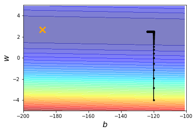
plt.show()

作出如下图一，黑色线代表参数求解的迭代路径。假设我们已经知道实际最优解的位置在橘色叉叉$(-188.4，2.67)$处，现在考察用梯度下降法求解出来的参数，与这个实际最优解$(-188.4，2.67)$相差多大。图一中，我们设定初始参数的出发位置为$(b，w) = (-120，-4)$，学习率为$0.0000001$，迭代次数为$100000$次，解得参数$(b，w) = (-123.69，2.48)$，这个解与实际最优解相差很远。

图一：lr=0.0000001，iteration=100000，(b，w)=(-123.69，2.48)

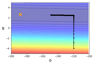
为了求得最佳参数，尝试使迭代次数保持不变（$100000$次），学习率分别增大10倍，设为$0.000001$、$0.00001$。

图二：lr=0.000001，iteration=100000，(b，w)=(-149.23， 2.56)

图三：lr=0.00001，iteration=100000，(b，w)=(nan，nan)

图三学习率过大，严重偏离最优解的迭代路径，参数已经变成NA值。
故尝试使学习率保持不变（$0.0000001$），迭代次数分别设为$1000000$、$10000000$。图五可见迭代效果不错，但迭代次数很大。

图四：lr=0.0000001，iteration=1000000，(b，w)=(-149.23，2.56)

图五：lr=0.0000001，iteration=10000000，(b，w)=(-188.17，2.67)

---

Adagrad优化算法

虽然图五通过增加迭代次数，逐渐逼近最优参数，但是运行的时间也相应增加。考虑用Adagrad优化算法：在迭代过程中，分别对参数$w$、$b$指定客制化的学习率。

import numpy as np
import matplotlib.pyplot as plt


x_data = [338, 333, 328, 207, 226, 25, 179, 60, 208, 606]
y_data = [640, 633, 619, 393, 428, 27, 193, 66, 226, 1591]


x = np.arange(-200, -100)
y = np.arange(-5, 5, 0.1)
Z = np.zeros((len(x), len(y)))
X, Y = np.meshgrid(x, y)
for i in range(len(x)):                      
    for j in range(len(y)):
        b = x[i]
        w = y[j]
        Z[j][i] = 0
        for n in range(len(x_data)):
            Z[j][i] += (y_data[n] - b - w * x_data[n]) ** 2
        Z[j][i] = Z[j][i] / len(x_data)


b = -120
w = -4
lr = 1                                 # 学习率随便设为1
iteration = 100000


b_history = [b]
w_history = [w]
lr_b = 0                               # 参数b的初始学习率为0
lr_w = 0                               # 参数w的初始学习率为0

for i in range(iteration):
    b_grad = 0.0                                                         
    w_grad = 0.0                                                         
    for n in range(len(x_data)):
        b_grad -= 2.0 * (y_data[n] - b - w * x_data[n]) * 1.0           # L对参数b的偏导值    
        w_grad -= 2.0 * (y_data[n] - b - w * x_data[n]) * x_data[n]     # L对参数w的偏导值

    # 偏导数累加
    lr_b = lr_b + b_grad ** 2                                          
    lr_w = lr_w + w_grad ** 2

    # 用Adagrad的学习率更新参数
    b = b - lr/np.sqrt(lr_b) * b_grad
    w = w - lr/np.sqrt(lr_w) * w_grad

    b_history.append(b)
    w_history.append(w)


plt.contourf(x, y, Z, 50, alpha=0.5, cmap=plt.get_cmap('jet'))
plt.plot([-188.4], [2.67], 'x', ms=12, markeredgewidth=3, color='orange')
plt.plot(b_history, w_history, 'o-', ms=3, lw=1.5, color='black')
plt.xlim(-200, -100)
plt.ylim(-5, 5)
plt.xlabel(r'$b$', fontsize=16)
plt.ylabel(r'$w$', fontsize=16)
plt.show()

解得最优参数为$(b，w)=(-188.37，2.67)$。

---

相关Python函数

range(start, stop, step)
# 起始值为start（默认从0开始），结束值为stop（不包括stop本身），step为间距
# 结果生成一个range对象，而不是一个数值序列
[In]: range(5) == range(0, 5)
[Out]: True
[In]: c = [i for i in range(5)];print(c)
[Out]: [0, 1, 2, 3, 4]


import numpy as np
np.arange(start, stop, step)
# 起始值为start（默认从0开始），结束值为stop（不包括stop本身），step为间距
# 结果生成一个array，数值序列
[In]: x = np.arange(0, 2);y = np.arange(0, 5);print(x);print(y)
[Out]:
[0 1]
[0 1 2 3 4]


np.zeros(shape, dtype=float, order='C')
# 参数shape为数值或数值序列，设定array的形状
# 参数dtype表示数据类型，默认numpy.float64；参数order可选'C'（行优先）或'F'（列优先）
# 返回一个填充0值的array
[In]: np.zeros(shape=(2,5))
[Out]: 
array([[0., 0., 0., 0., 0.],
       [0., 0., 0., 0., 0.]])
# 生成2×5的array


np.meshgrid(x, y)
# 参数x和y是一维向量，x中的值作为横坐标（做竖向扩展），y中的值作为纵坐标（做横向扩展）
# 结果返回一个坐标矩阵（网格矩阵）
[In]: x = np.arange(0, 2);y = np.arange(0, 5);print(x);print(y)
[Out]:
[0 1]
[0 1 2 3 4]
[In]: X, Y = np.meshgrid(x, y);print(X);print(Y)
[Out]:
[[0 1]
 [0 1]
 [0 1]
 [0 1]
 [0 1]]
[[0 0]
 [1 1]
 [2 2]
 [3 3]
 [4 4]]
 # X、Y均是5×2的array
 # 可见，向量x竖向扩展了len(y)次，向量y横向扩展了len(x)次，X和Y这两个array的行列数是相同的