Lecture note 3: Linear and Logistic Regression in TensorFlow #
之前的学习内容:
Graphs and sessions
TF Ops: constants, variables, functions
TensorBoard!
Lazy loading
1. Linear Regression in TensorFlow
让我们先从一个简单的线性回归的例子开始。我希望你已经熟悉线性回归,如果没有的话,你可以在维基百科中查看。
问题:我们经常听到保险公司使用诸如火灾和盗窃之类的因素来计算社区的危险程度。
我的问题是:这是多余的吗?
在一个社区里,火灾和盗窃的数量是否有关系,如果有的话,我们能找到它吗?
换句话说,我们能否找到一个函数f如果X是火灾的数量而Y是偷窃的数量,那么Y=f(X)?
考虑到这段关系,如果我们有一个特定区域的火灾数量,我们能预测那个地区的盗窃次数。
我们有由美国公民权利委员会收集的数据,这是由 Cengage Learning提供的。
数据集描述:
Nname:在芝加哥的火灾和盗窃
X:每1000个住宅单位的火灾数量
Y:在芝加哥市区的同一邮政编码区,每1000名居民的偷窃行为。
邮政编码区域总数:42
解决方案:首先,假设火灾和偷窃的数量之间的关系是线性的:Y=wX+b
我们需要找到标量参数w和b,用均值平方误差作为损失函数。
我们写程序。
import numpy as np
import matplotlib.pyplot as plt
import tensorflow as tf import xlrd
DATA_FILE = "data/fire_theft.xls"
# Step 1: read in data from the .xls file
book = xlrd.open_workbook(DATA_FILE, encoding_override="utf-8")
sheet = book.sheet_by_index(0)
data = np.asarray([sheet.row_values(i) for i in range(1, sheet.nrows)])
n_samples = sheet.nrows - 1
# Step 2: create placeholders for input X (number of fire) and label Y (number of theft)
X = tf.placeholder(tf.float32, name="X")
Y = tf.placeholder(tf.float32, name="Y")
# Step 3: create weight and bias, initialized to 0
w = tf.Variable(0.0, name="weights")
b = tf.Variable(0.0, name="bias")
# Step 4: construct model to predict Y (number of theft) from the number of fire
Y_predicted = X * w + b
# Step 5: use the square error as the loss function
loss = tf.square(Y - Y_predicted, name="loss")
# Step 6: using gradient descent with learning rate of 0.01 to minimize loss
optimizer = tf.train.GradientDescentOptimizer(learning_rate=0.001).minimize(loss)
with tf.Session() as sess:
# Step 7: initialize the necessary variables, in this case, w and b sess.
run(tf.global_variables_initializer())
# Step 8: train the model for i in range(100): # run 100 epochs
for x, y in data: # Session runs train_op to minimize loss
sess.run(optimizer, feed_dict={X: x, Y:y})
# Step 9: output the values of w and b w_value, b_value = sess.run([w, b])
经过100次的训练后,我们的平均损失为1372.77701716,而w=1.62071,b=16.9162。
损失相当大。
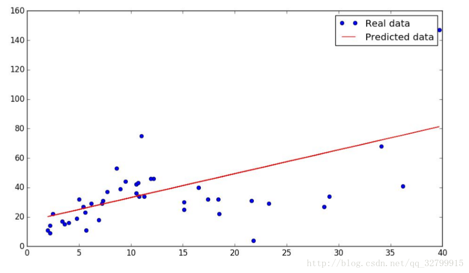
它并不适合。我们能更好地利用二次函数Y=wXX+uX+b吗?让我们试一试。我们只需要添加另一个变量u,然后改变y预测值的公式。
# Step 3: create variables: weights_1, weights_2, bias. All are initialized to 0
w = tf.Variable(0.0, name="weights_1")
u = tf.Variable(0.0, name="weights_2")
b = tf.Variable(0.0, name="bias")
# Step 4: predict Y (number of theft) from the number of fire
Y_predicted = X * X * w + X * u + b
# Step 5: Profit!
经过100次的训练后,我们的平均损失为797.335975976 , w, u, b = [0.071343 0.010234 0.00143057]
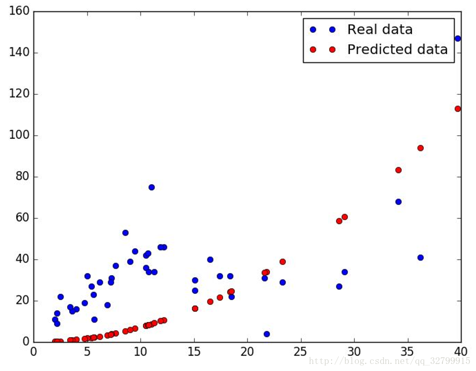
这比线性函数收敛的时间要少,但由于右侧的几个异常值,仍然完全关闭。
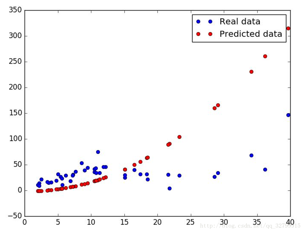
它可能会更好地在Huber的损失中,而不是MSE或第三个多项式,作为函数f,你自己尝试。
使用Huber的二次模型,我得到了一些更好的东西,忽略了异常值:
我们怎么知道我们的模型是正确的呢?
使用相关系数r平方
以防你不知道r-平方是什么,Minitab有一个很好的博客文章在这里解释。
下面是它的要点:“r-平方是一种统计数据,用来衡量数据与拟合回归线的距离。
它也被称为确定系数,或者多重回归的多重确定系数。
r平方的定义是相当直接的;
它是由线性模型解释的响应变量变化的百分比。
R-squared=Explained variation/Total variation
在测试集中运行
我们在机器学习课上学到的是,这一切都归结于验证和测试。
因此,第一个方法显然是在测试集上测试我们的模型。
为训练、验证和测试提供单独的数据集是非常棒的,但是这意味着我们将有更少的训练数据。
有很多文献可以帮助我们绕过那些没有大量数据的案例,比如k-折叠交叉验证
用虚拟数据测试我们的模型
我们可以测试模型的另一种方法是对虚拟数据进行测试。
例如,在这种情况下,我们可以创建一些虚拟数据,这些数据的线性关系已经知道了,可以测试我们的模型。
在这种情况下,让我们创建100个数据点(X,Y)这样的Y~3*X,看看我们的模型输出w=3 b=0。
生成虚拟数据:
# each value y is approximately linear but with some random noise
X_input = np.linspace(-1, 1, 100)
Y_input = X_input * 3 + np.random.randn(X_input.shape[0]) * 0.5
我们使用numpy数组X_input和Y_input,以支持稍后的迭代(当我们输入占位符X和Y时)。
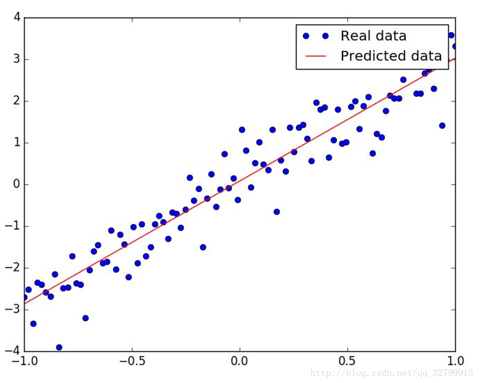
它拟合得很好!
这个故事的寓意:虚拟数据比真实世界数据要容易得多,因为虚拟数据是根据模型的假设生成的。
现实世界是艰难的!
分析代码
我们的模型中的代码非常简单,除了两行:
optimizer = tf.train.GradientDescentOptimizer(learning_rate=0.01).minimize(loss)
sess.run(optimizer, feed_dict={X: x, Y:y})
我记得我第一次遇到类似的代码时,我很困惑。两个问题:
1.
为什么在tf.session.run()的获取列表中进行训练?
2.
TensorFlow如何知道要更新哪些变量?
实际上,我们可以在tf.session.run()中传递任何TensorFlow操作。
TensorFlow将执行这些操作所依赖的图形的一部分。
在这种情况下,我们看到训练的目的是最小化损失,而损失则取决于变量w和b。
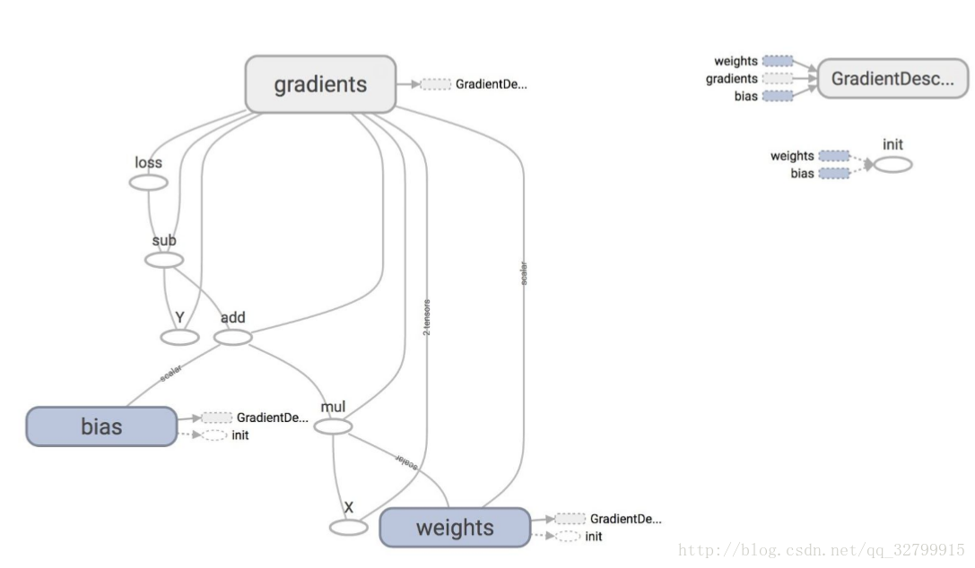
从图中,可以看到巨大的节点GrandientDescentOptimizer取决于三个节点:权重,偏置,和梯度。
优化器 Optimizers
梯度下降优化意味着我们的更新规则是梯度下降。
TensorFlow自动进行微分,然后更新w和b的值以最小化损失。
Autodiff是惊人的!
在默认情况下,优化器将训练所有可训练的变量,它们的目标函数依赖于这些变量。
如果有一些你不想训练的变量,那么当你声明一个变量时,你可以将关键字训练设置为False。
你不想训练的变量的一个例子是变量globalstep,这是一个常见的变量,你将在许多TensorFlow模型中看到,以跟踪你运行模型的次数。
global_step = tf.Variable(0, trainable=False, dtype=tf.int32
learning_rate = 0.01 * 0.99 ** tf.cast(global_step, tf.float32)

increment_step = global_step.assign_add(1)
optimizer = tf.GradientDescentOptimizer(learning_rate)
# learning rate can be a tensor
在我们讨论的时候,让我们看一下tf.Variable变量的完整定义:
tf.Variable(initial_value=None, trainable=True, collections=None, validate_shape=True, caching_device=None, name=None, variable_def=None, dtype=None, expected_shape=None, import_scope=None)
你还可以要求优化器使用特定变量的梯度。你还可以修改由优化器计算的梯度。
# create an optimizer.
optimizer = GradientDescentOptimizer(learning_rate=0.1)
# compute the gradients for a list of variables.
grads_and_vars = opt.compute_gradients(loss, <list of variables>)
# grads_and_vars is a list of tuples (gradient, variable). Do whatever you # need to the 'gradient' part, for example, subtract each of them by 1.
subtracted_grads_and_vars = [(gv[0] - 1.0, gv[1]) for gv in grads_and_vars]
# ask the optimizer to apply the subtracted gradients.
optimizer.apply_gradients(subtracted_grads_and_vars)
计算梯度
优化器类会自动在图上计算导数,但是新优化器或专家用户的创建者可以调用下面的底层函数。
tf.gradients(ys, xs, grad_ys=None, name='gradients', colocate_gradients_with_ops=False, gate_gradients=False, aggregation_method=None)
这个方法构造了ys和的偏导数符号,关于xs中的x。
ys和xs都是张量或张量的list。
grad_ys是一个张量list,它保存着ys接收到的梯度。
这个list必须与ys的长度相同。
技术细节:这在训练部分模型时特别有用。
例如,我们可以使用tf.gradients()来将损失的导数传播到中间层。
然后我们使用优化器来最小化中间层输出M和M+G之间的差异,这只会更新网络的下半部分。
优化器列表
梯度下降优化器不是TensorFlow支持的唯一更新规则。
这是TensorFlow支持的优化器列表,截止到2017年1/8。
名字都是不言而喻的。
你可以访问官方文档了解更多细节:
tf.train.GradientDescentOptimizer
tf.train.AdadeltaOptimizer
tf.train.AdagradOptimizer
tf.train.AdagradDAOptimizer
tf.train.MomentumOptimizer
tf.train.AdamOptimizer
tf.train.FtrlOptimizer
tf.train.ProximalGradientDescentOptimizer
tf.train.ProximalAdagradOptimizer
tf.train.RMSPropOptimizer
Sebastian Ruder是数据分析研究中心的博士候选人,他在他的博客文章中对这些优化器进行了比较。
如果你懒得阅读,以下是结论:
RMSprop是Adagrad的一个扩展,它可以使学习速度的急剧下降。
它与Adadelta是相同的,除了Adadelta在分子更新规则中使用了参数更新的RMS。
最后,Adam 补充了“bias-correction”偏置修正和“momentum”动量对RMSprop。
在这种情况下,RMSprop、Adadelta和Adam都是非常相似的算法。
Kingma等显示,它的“修正”帮助Adam在优化结束时略微超越了Adadelta,因为梯度变得稀疏。
在这一问题上,Adam可能是最好的选择。”
讨论问题
我们可以用线性回归解决哪些实际问题呢?
你能写一个快速的程序吗?
在TensorFlow逻辑回归
如果没有逻辑回归,我们就不能讨论线性回归。
让我们来解释一下TensorFlow中的逻辑回归,它解决了MNIST数据库中的分类问题。
MNIST数据库(混合国家标准和技术数据库)可能是用于训练各种图像处理系统的最流行的数据库之一,它是一个手写数字的数据库。
图像是这样的:
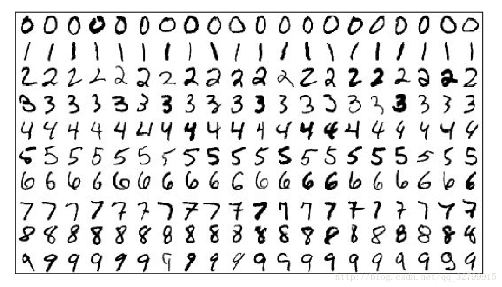
每个图像都是28 x 28像素,为1-d张量,大小为784。每一个都有一个标签。
例如,第一行上的图像被标记为0,第二个为1,以此类推。数据托管在 Yann Lecun的网站上(http://yann.lecun.com/exdb/mnist/)。
TFLearn(TensorFlow的简化界面)有一个脚本,让你从Yann Lecun的网站上加载MNIST的数据集,并把它分成训练集、验证集和测试集。
from tensorflow.examples.tutorials.mnist import input_data
MNIST = input_data.read_data_sets("/data/mnist", one_hot=True)
MNIST是一个TensorFlow的数据集对象。
它有15,000个数据(mnist.train),10,000个的测试数据(mnist.test),以及5000个的验证数据(mnist.validation)。
逻辑回归模型的构建与线性回归模型非常相似。然而,现在我们有了更多的数据。我们在CS229中学到了,如果我们在每一个数据点之后计算梯度,它将会非常缓慢。解决这个问题的一种方法是将它们进行批量处理。
幸运的是,TensorFlow对批处理数据有很好的支持。为了进行批处理逻辑回归,我们只需要更改x占位符和y占位符的维度,以便能够容纳不同大小的数据。
X = tf.placeholder(tf.float32, [batch_size, 784], name="image")
Y = tf.placeholder(tf.float32, [batch_size, 10], name="label")
当你将数据输入到占位符时,而不是为每个数据点提供数据,我们可以根据数据点的数量来提供数据。
X_batch, Y_batch = mnist.test.next_batch(batch_size)
sess.run(train_op, feed_dict={X: X_batch, Y:Y_batch})
这是完整的实现
import time import numpy as np
import tensorflow as tf
from tensorflow.examples.tutorials.mnist import input_data
# Step 1: Read in data
# using TF Learn's built in function to load MNIST data to the folder data/mnist
MNIST = input_data.read_data_sets("/data/mnist", one_hot=True)
# Step 2: Define parameters for the model
learning_rate = 0.01
batch_size = 128
n_epochs = 25
# Step 3: create placeholders for features and labels
# each image in the MNIST data is of shape 28*28 = 784
# therefore, each image is represented with a 1x784 tensor
# there are 10 classes for each image, corresponding to digits 0 - 9.
# each label is one hot vector.
X = tf.placeholder(tf.float32, [batch_size, 784])
Y = tf.placeholder(tf.float32, [batch_size, 10])
# Step 4: create weights and bias
# w is initialized to random variables with mean of 0, stddev of 0.01
# b is initialized to 0
# shape of w depends on the dimension of X and Y so that Y = tf.matmul(X, w)
# shape of b depends on Y
w = tf.Variable(tf.random_normal(shape=[784, 10], stddev=0.01), name="weights")
b = tf.Variable(tf.zeros([1, 10]), name="bias")
# Step 5: predict Y from X and w, b
# the model that returns probability distribution of possible label of the image
# through the softmax layer
# a batch_size x 10 tensor that represents the possibility of the digits
logits = tf.matmul(X, w) + b
# Step 6: define loss function
# use softmax cross entropy with logits as the loss function
# compute mean cross entropy, softmax is applied internally
entropy = tf.nn.softmax_cross_entropy_with_logits(logits, Y)
loss = tf.reduce_mean(entropy)
# computes the mean over examples in the batch
# Step 7: define training op
# using gradient descent with learning rate of 0.01 to minimize cost
optimizer = tf.train.GradientDescentOptimizer(learning_rate=learning_rate).minimize(loss)
init = tf.global_variables_initializer()
with tf.Session() as sess:
sess.run(init)
n_batches = int(MNIST.train.num_examples/batch_size)
for i in range(n_epochs):
# train the model n_epochs times
for _ in range(n_batches):
X_batch, Y_batch = MNIST.train.next_batch(batch_size)
sess.run([optimizer, loss], feed_dict={X: X_batch, Y:Y_batch})
# average loss should be around 0.35 after 25 epochs
运行在我的Mac上,批量大小128的模型在0.5秒内运行,而非批处理模型在24秒内运行!
但是,请注意,较高的批处理大小通常需要更多的时间,因为它执行的更新步骤更少。
在Bengio的实用技巧中,可以看到“迷你批量”。
我们可以测试这个模型因为我们有一个测试集,让我们看看如何在TensorFlow中完成它。
# test the model
n_batches = int(MNIST.test.num_examples/batch_size)
total_correct_preds = 0
for i in range(n_batches):
X_batch, Y_batch = MNIST.test.next_batch(batch_size)
_, loss_batch, logits_batch = sess.run([optimizer, loss, logits], feed_dict={X: X_batch, Y:Y_batch})
preds = tf.nn.softmax(logits_batch)
correct_preds = tf.equal(tf.argmax(preds, 1), tf.argmax(Y_batch, 1)) accuracy = tf.reduce_sum(tf.cast(correct_preds, tf.float32)) # similar
to numpy.count_nonzero(boolarray) :( total_correct_preds += sess.run(accuracy)
print "Accuracy {0}".format(total_correct_preds/MNIST.test.num_examples)
在10个迭代之后,我们的准确率达到了90%。这就是我们从线性分类器中得到的。
注意:TensorFlow为MNIST提供了一个feeder(数据集解析器),但不要指望它为任何数据集提供一个feeder。
您应该学习如何编写自己的数据解析器。
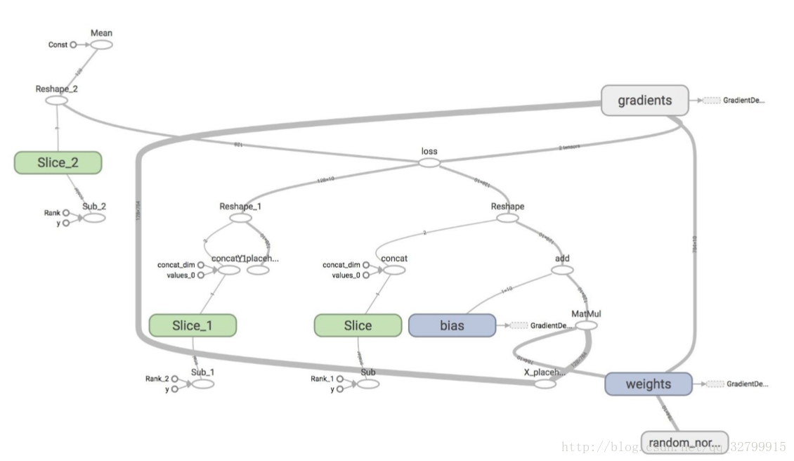
这是我们的图表在TensorBoard上的样子
我知道。
这就是为什么我们会在下节课学习如何构建模型的原因。