文章目录
1.前言
解决分类问题里最普遍的baseline model就是逻辑回归,简单同时可解释性好,使得它大受欢迎,我们来用tensorflow完成这个模型的搭建。
在这篇文章中我们使用的是MNIST手写数字识别图像的数据集。
模型搭建的步骤和代码如下:
2.程序详细讲解
环境设定
import numpy as np
import tensorflow as tf
from tensorflow.examples.tutorials.mnist import input_data
import time
数据读取
#使用tensorflow自带的工具来加载MNIST手写数字集合
mnist = input_data.read_data_sets('./data/mnist', one_hot=True)
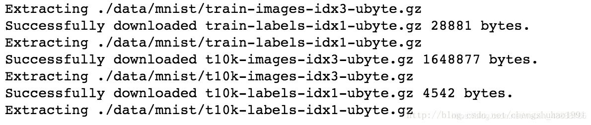
上图即表示数据读取加载完成,后面我们可以查看一下数据的基本信息。
#查看一下数据维度
mnist.train.images.shape

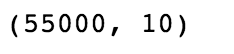
#查看target维度
mnist.train.labels.shape
准备好placeholder,开好容器来装数据
batch_size = 128     #指定每次传入进内存的数据大小,指定之后可以防止数据出现错误
X = tf.placeholder(tf.float32, [batch_size, 784], name='X_placeholder')
Y = tf.placeholder(tf.int32, [batch_size, 10], name='Y_placeholder')

#其实可以用下面这种方式,在不知道数据集大小的时候,传入的数据大小不固定,后面再根据实际情况来指定
# X = tf.placeholder(tf.float32, [None, 784], name='X_placeholder')
# Y = tf.placeholder(tf.int32, [None, 10], name='Y_placeholder')
准备好参数/权重
此处准备参数时一定要将参数的维度设定好,不然后面的计算会出错误。
w = tf.Variable(tf.random_normal(shape=[784, 10], stddev=0.01), name='weights')
b = tf.Variable(tf.zeros([1, 10]), name="bias")
拿到每个类别的score
logits = tf.matmul(X, w) + b
计算多分类softmax的loss function
# 求交叉熵损失
entropy = tf.nn.softmax_cross_entropy_with_logits(logits=logits, labels=Y, name='loss')
# 求平均
loss = tf.reduce_mean(entropy)    #此处使用的是求平均值的方式
准备好optimizer
这里的最优化用的是随机梯度下降,我们可以选择AdamOptimizer这样的优化器。Adam.Optimiter()是一个带动量的梯度下降,不会很快陷到局部最低点,它会找到一个接近全局最优解的低点,但不保证会找到全局最优解.
learning_rate = 0.01
optimizer = tf.train.AdamOptimizer(learning_rate).minimize(loss)
在session里执行graph里定义的运算
#迭代总轮次
n_epochs = 30

with tf.Session() as sess:
    # 在Tensorboard里可以看到图的结构
    writer = tf.summary.FileWriter('./graphs/logistic_reg', sess.graph)

    start_time = time.time()
    sess.run(tf.global_variables_initializer())
    n_batches = int(mnist.train.num_examples/batch_size)
    for i in range(n_epochs): # 将所有的训练数据迭代这么多轮
        total_loss = 0

        for _ in range(n_batches):
            X_batch, Y_batch = mnist.train.next_batch(batch_size)
            _, loss_batch = sess.run([optimizer, loss], feed_dict={X: X_batch, Y:Y_batch})
            total_loss += loss_batch
        print('Average loss epoch {0}: {1}'.format(i, total_loss/n_batches))

    print('Total time: {0} seconds'.format(time.time() - start_time))

    print('Optimization Finished!')
由于此数据集有测试集,不同于上面两篇文章中自己生成的数据,因此需要用测试集来测试模型的准确率
    # 测试模型,也需要放到session里面来运行。

    preds = tf.nn.softmax(logits)   #通过softmax()来计算每个样本类别的概率值
    correct_preds = tf.equal(tf.argmax(preds, 1), tf.argmax(Y, 1))   #此处得出的是一个一阶张量,由一串0,1数字组成,表示的是每个样本是否预测预测准确
    accuracy = tf.reduce_sum(tf.cast(correct_preds, tf.float32))  #对预测是否准确的列表求平均值 ,cast()函数是将整型数据转化为浮点型数据

    n_batches = int(mnist.test.num_examples/batch_size) #输入数据的批次
    total_correct_preds = 0

    #对测试集每个batch求accuracy
    for i in range(n_batches):
        X_batch, Y_batch = mnist.test.next_batch(batch_size)    #此处是从测试集中按批次的输入数据
        accuracy_batch = sess.run([accuracy], feed_dict={X: X_batch, Y:Y_batch})
        total_correct_preds += accuracy_batch[0]
    #对每个batch求平均值
    print('Accuracy {0}'.format(total_correct_preds/mnist.test.num_examples))

    writer.close()
3.总代码
# -*- coding: utf-8 -*-
'''
A logistic regression learning algorithm example using TensorFlow library.
This example is using the MNIST database of handwritten digits
(http://yann.lecun.com/exdb/mnist/)
Author: Aymeric Damien
Project: https://github.com/aymericdamien/TensorFlow-Examples/
'''
from __future__ import print_function
import tensorflow as tf
# Import MNIST data(下载数据)
from tensorflow.examples.tutorials.mnist import input_data
mnist = input_data.read_data_sets("/tmp/data/", one_hot=True)
# 参数:学习率,训练次数,
learning_rate = 0.01
training_epochs = 25
batch_size = 100
display_step = 1
# tf Graph Input
x = tf.placeholder(tf.float32, [None, 784]) # mnist data image of shape 28*28=784
y = tf.placeholder(tf.float32, [None, 10]) # 0-9 digits recognition => 10 classes
# Set model weights
W = tf.Variable(tf.zeros([784, 10]))
b = tf.Variable(tf.zeros([10]))
# softmax模型
pred = tf.nn.softmax(tf.matmul(x, W) + b) # Softmax
# Minimize error using cross entropy(损失函数用cross entropy)
cost = tf.reduce_mean(-tf.reduce_sum(y*tf.log(pred), reduction_indices=1))
# Gradient Descent(梯度下降优化)
optimizer = tf.train.GradientDescentOptimizer(learning_rate).minimize(cost)
# Initializing the variables
init = tf.global_variables_initializer()
# Launch the graph
with tf.Session() as sess:
sess.run(init)
# Training cycle
for epoch in range(training_epochs):
avg_cost = 0.
total_batch = int(mnist.train.num_examples/batch_size)
# Loop over all batches
for i in range(total_batch):
batch_xs, batch_ys = mnist.train.next_batch(batch_size)
# Run optimization op (backprop) and cost op (to get loss value)
_, c = sess.run([optimizer, cost], feed_dict={x: batch_xs,
y: batch_ys})
# Compute average loss
avg_cost += c / total_batch
# Display logs per epoch step
if (epoch+1) % display_step == 0:
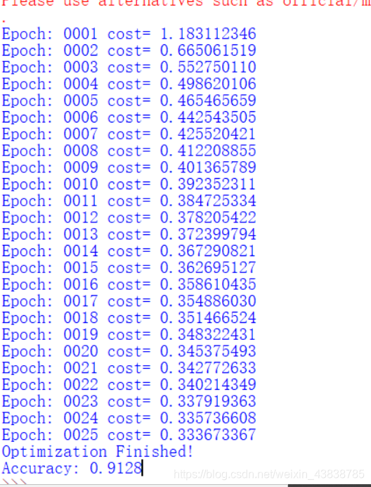
print("Epoch:", '%04d' % (epoch+1), "cost=", "{:.9f}".format(avg_cost))
print("Optimization Finished!")
# Test model
correct_prediction = tf.equal(tf.argmax(pred, 1), tf.argmax(y, 1))
# Calculate accuracy
accuracy = tf.reduce_mean(tf.cast(correct_prediction, tf.float32))
print("Accuracy:", accuracy.eval({x: mnist.test.images, y: mnist.test.labels}))
4.输出结果
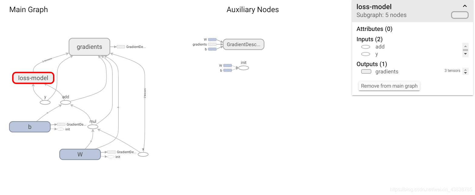
5.可视化
使用tensorBoard方法 在这片文章中
https://blog.csdn.net/weixin_43838785/article/details/104433504
Scalars
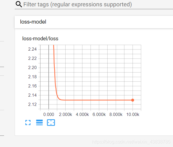
2.00k次左右已经稳定
Graphs