05_Support Vector Machines_02_Polynomial Kernel_Gaussian RBF_Kernelized SVM Regression_Quadratic Pro

05_Support Vector Machines_hinge_support vectors_decision function_Lagrange multiplier拉格朗日乘数https://blog.csdn.net/Linli522362242/article/details/104151351

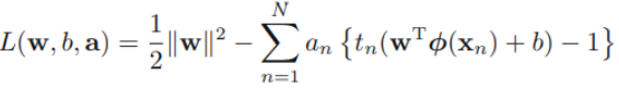
Using these results to eliminate w, b, and {ξn} from the Lagrangian, we obtain the dual Lagrangian in the form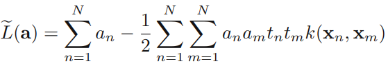
 
which is identical to the separable case(7.10), except that the constraints are somewhat different. To see what these constraints are, we note that  is required because these are Lagrange multipliers. Furthermore, (7.31) together with  implies an We therefore have to minimize (7.32) with respect to the dual variables {} subject to

for n = 1,...,N, where (7.33) are known as box constraints. This again represents a quadratic programming problem. If we substitute (7.29) into (7.1), we see that predictions for new data points are again made by using (7.13).

We can now interpret the resulting solution. As before, a subset of the data points may have  = 0, in which case they do not contribute to the predictive model (7.13 ). The remaining data points constitute the support vectors since these have  and hence from (7.25: ) must satisfy

If  < C, then (7.31 ) implies that  > 0, which from (7.28) requires ξn = 0 and hence such points lie on the margin. Points with  = C can lie inside the margin and can either be correctly classified if  or misclassified if ξn > 1. 

Hinge损失函数
https://blog.csdn.net/Linli522362242/article/details/104151351

sub-Summary: to solve 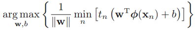  #### SVM (Maximum Margin Classifiers)
-->At first,   since the constraints , so the minimum value is 1 which is lead by the support vectors(find them at first)

Then maximize  ==> maximize ==> is equivalent to minimizing ==>    #The factor of is included for computation convenience.
 

  对线性SVM分类器来说，方法之一是使用梯度下降，使从原始问题导出的成本函数最小化。线性SVM分类器cost function成本函数：
                            vs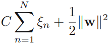  
成本函数中的第一项会推动模型得到一个较小的权重向量w，从而使间隔更大。
在第二项中的1表示间隔（margin）大小, 并且 此成本函数的C 的符号与 右边成本函数（slack）前的C的符号是相反的（由于1-t*y==-slack = -ξn）; 换句话说在 sklearn中的hinge loss的C 前面是负号

第二项则计算全部的间隔违例。如果没有一个示例位于街道之上，并且都在街道正确的一边，那么这个实例的间隔违例为0；如不然，则该实例的违例大小与其到街道正确一边的距离成正比。所以将这个项最小化，能够保证模型使间隔违例尽可能小，也尽可能少。
函数被称为hinge损失函数（如下图所示）。其中，t为目标值 class label（-1或+1），y是分类器输出的预测值 ，并不直接是类标签。其含义为，当t和y的符号相同时（表示y预测正确）并且|y|≥1时，hinge loss为0；当t和y的符号相反时，hinge loss随着y的增大线性增大。
　　Hinge loss用于最大间隔（maximum-margin）分类，其中最有代表性的就是支持向量机SVM。

　　Hinge函数的标准形式：

（与上面统一的形式：）
但是它还有一个smoothed versions: https://en.wikipedia.org/wiki/Hinge_loss

if we use slack variables to represent hinge loss: 1-t*y==-slack = -ξn

with ξn > 1 will be misclassified. The exact classification constraints (7.5: ) are then replaced with   
in which the slack variables are constrained to satisfy . Data points for which ξn = 0 are correctly classified and are either on the margin or on the correct side of the margin. Points for which   lie inside the margin, but on the correct side of the decision boundary(In hinge loss, here's slack ξn is also 0), and those data points for which ξn > 1 lie on the wrong side of the decision boundary and are misclassified, as illustrated in Figure 7.3. This is sometimes described as relaxing the hard margin constraint to give a soft margin and allows some of the training set data points to be misclassified. Note that while slack variables allow for overlapping class distributions, this framework is still sensitive to outliers because the penalty for misclassification increases linearly with ξ.

Our goal is now to maximize the margin while softly penalizing points that lie on the wrong side of the margin boundary. We therefore minimize             
where the parameter C > 0 controls the trade-off between the slack variable penalty and the margin. Because any point that is misclassified has ξn > 1, it follows that  is an upper bound on the number of misclassified points. The parameter C is therefore analogous相似的 to (the inverse of) a regularization coefficient because it controls the trade-off between minimizing training errors and controlling model complexity. In the limit C → ∞, we will recover the earlier support vector machine for separable data.
a smaller C value leads to a wider street but more margin violations（too many ξn OR  too large, Note: we want to minimize the cost function or hinge loss）
a high C value the classifier makes fewer margin violations but ends up with a smaller margin
换句话说在 sklearn中的hinge loss的C 前面是号

scaler = StandardScaler() 
svm_clf1 = LinearSVC( C=1, loss="hinge", random_state=42 ) 
svm_clf2 = LinearSVC( C=100, loss="hinge", random_state=42 )

Polynomial Kernel

Adding polynomial features is simple to implement and can work great with all sorts of Machine Learning algorithms (not just SVMs), but at a low polynomial degree it cannot deal with very complex datasets, and with a high polynomial degree it creates a huge number of features, making the model too slow.

Fortunately, when using SVMs you can apply an almost miraculous神奇的 mathematical technique called the kernel trick (it is explained in a moment). It makes it possible to get the same result as if you added many polynomial features, even with very highdegree polynomials, without actually having to add them. So there is no combinatorial explosion组合爆炸 of the number of features since you don’t actually add any features. This trick is implemented by the SVC class. Let’s test it on the moons dataset:

https://blog.csdn.net/Linli522362242/article/details/104070847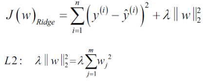
 or 

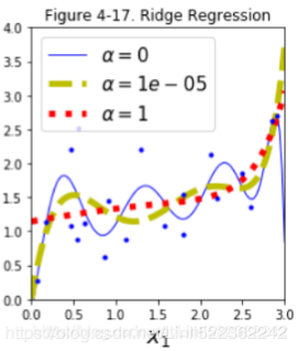
plot_model(Ridge, polynomial=True, alphas=(0,10**-5, 1), random_state=42)

If α = 0 then Ridge Regression is just polynomial Linear Regression(overfitting). 
If α is very large(e.g. α=1), then all weights end up  very close to zero and the result is a flat line going through the data's mean(better than α = 0)

By increasing the value of the hyperparameter  (or uses ), we increase the regularization strength(for tackling the problem of overfitting) and shrink the weights of our model(or reduce the value of wj or bj) since we want to make the function attain the minimum( including ).  Note sometimes the value of wj or theta_i  is not steady or maybe too large.  If α is very large, then all weights end up very close to zero

 |  C : float, optional (default=1.0)
 |      Regularization parameter. The strength of the regularization is
 |      inversely proportional to C. Must be strictly positive. The penalty
 |      is a squared l2 penalty.

This code trains an SVM classifier using a 3rd-degree polynomial kernel. It is represented on the left of Figure 5-7. On the right is another SVM classifier using a 10th-degree polynomial kernel. Obviously, if your model is overfitting, you might want to reduce the polynomial degree. Conversely, if it is underfitting, you can try increasing it. The hyperparameter coef0 controls how much the model is influenced by high-degree polynomials versus low-degree polynomials.

The hyperparameter coef0 controls how much the model is influenced by high-degree polynomials

from sklearn.svm import SVC

poly_kernel_svm_clf = Pipeline([
    ("scaler", StandardScaler()),             #######
    ("svm_clf", SVC(kernel="poly", degree=17, coef0=1, C=5)),
])

#X,y = make_moons(n_samples=100, noise=0.15, random_state=42)
poly_kernel_svm_clf.fit(X,y)

from sklearn.svm import SVC

poly100_kernel_svm_clf = Pipeline([
    ("scaler", StandardScaler()),             #########
    ("svm_clf", SVC(kernel="poly", degree=17, coef0=100, C=5))
])

poly100_kernel_svm_clf.fit(X,y)



fig, axes = plt.subplots(ncols=2, figsize=(10.5, 4), sharey=True)

plt.sca(axes[0])
plot_predictions(poly_kernel_svm_clf, [-1.5,2.45, -1,1.5])
plot_dataset(X, y, [-1.5,2.4, -1,1.5])
plt.title(r"$d=17, r=1, C=5$", fontsize=18)

plt.sca(axes[1])
plot_predictions(poly100_kernel_svm_clf, [-1.5,2.45, -1,1.5])
plot_dataset(X,y, [-1.5,2.4, -1,1.5])
plt.title(r"$d=17, r=100, C=5$", fontsize=18)
plt.ylabel("")
plt.show()

The d=17 leaded the overfitting(see left figure), but increase the r(coef0=100) could reduce the influence from high-degree polynomial(right figure is better than left figure)

The hyperparameter coef0 controls how much the model is influenced by high-degree polynomials versus low-degree polynomials.

from sklearn.svm import SVC

poly_kernel_svm_clf = Pipeline([
    ("scaler", StandardScaler()),  #################
    ("svm_clf", SVC(kernel="poly", degree=3, coef0=1, C=5)),
])

#X,y = make_moons(n_samples=100, noise=0.15, random_state=42)
poly_kernel_svm_clf.fit(X,y)

from sklearn.svm import SVC

poly100_kernel_svm_clf = Pipeline([
    ("scaler", StandardScaler()),    ##################
    ("svm_clf", SVC(kernel="poly", degree=10, coef0=100, C=5))
])

poly100_kernel_svm_clf.fit(X,y)

fig, axes = plt.subplots(ncols=2, figsize=(10.5, 4), sharey=True)

plt.sca(axes[0])
plot_predictions(poly_kernel_svm_clf, [-1.5,2.45, -1,1.5])
plot_dataset(X, y, [-1.5,2.4, -1,1.5])
plt.title(r"$d=3, r=1, C=5$", fontsize=18)

plt.sca(axes[1])
plot_predictions(poly100_kernel_svm_clf, [-1.5,2.45, -1,1.5])
plot_dataset(X,y, [-1.5,2.4, -1,1.5])
plt.title(r"$d=10, r=100, C=5$", fontsize=18)
plt.ylabel("")
plt.show()

you saw that, the result of the d=10 is very similar to d=17; Besides, the result of the d=3 and r=1 is better than d=10, r=100(the result is overfiting,just little bit). so we need to find the right hyperparameter values.

A common approach to find the right hyperparameter values is to use grid search (see https://blog.csdn.net/Linli522362242/article/details/103646927). It is often faster to first do a very coarse grid search, then a finer grid search around the best values found. Having a good sense of what each hyperparameter actually does can also help you search in the right part of the hyperparameter space.

Adding Similarity Features

Another technique to tackle解决 nonlinear problems is to add features computed using a similarity function相似函数 that measures how much each instance resembles类似于 a particular landmark地标. For example, let's take the one-dimensional dataset discussed earlier and add two landmarks to it at x1 = –2 and x1 = 1 (see the left plot in Figure 5-8). Next, let’s define the similarity function to be the Gaussian Radial Basis Function (RBF)高斯辐射基函数 with γ = 0.3 (see Equation 5-1).
Equation 5-1. Gaussian RBF   OR 

######################### extra materials
The RBF kernel on two samples x and x', represented as feature vectors in some input space, is defined as

may be recognized as the squared Euclidean distance between the two feature vectors.  is a free parameter. An equivalent definition involves a parameter :   
Since the value of the RBF kernel decreases with distance and ranges between zero (in the limit) and one (when x = x'), it has a ready interpretation as a similarity measure.

why use Radial Basis Function kernel (RBF kernel)?

Supposing 100 samples (with two features each) will be assigned the class label 1 and 100 samples will be assigned the class label -1, respectively

Obviously, we would not be able to separate samples from the positive and negative class very well using a linear hyperplane as the decision boundary via the linear logistic regression or linear SVM model that we discussed in earlier sections.
The basic idea behind kernel methods to deal with such linearly inseparable data is to create nonlinear combinations of the original features to project them onto a higher dimensional space via a mapping function where it becomes linearly separable.
As shown in the next figure, we can transform a two-dimensional dataset(instances, 2features) onto a new three-dimensional feature space where the classes become separable via the following projection:
 
This allows us to separate the two classes shown in the plot via a linear hyperplane that becomes a nonlinear decision boundary if we project it back onto the original feature space: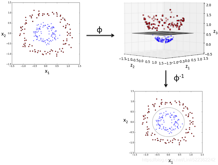

For models which are based on a fixed nonlinear feature space mapping , the kernel function is given by the relation
       
From this definition, we see that the kernel is a symmetric function of its arguments so that .

The simplest example of a kernel function is obtained by considering the identity mapping恒等映射 for the feature space in (6.1) so that = x, in which case . We shall refer to this as the linear kernel线性核.

Dual Representations对偶表示   SVM  Regresssion
##################extra

https://blog.csdn.net/Linli522362242/article/details/104070847
I suppose there is an instance with m-1 features,   =1, and the bias/intercept is ==
  
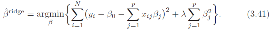
Then Ridge Regression cost function (= ,  = ,  is range of instances,  is range of features for each instance)
 =mean sum-of-square error +  L2 norm regularization term
 == 1/N *  * ,  where 
Note: is for convenient computation, , we should remove it for Practical application; 

https://blog.csdn.net/Linli522362242/article/details/104005906,
  as    and  is range of instances
   and 
 #   is range of instance; 
                                                              j is feature index,  each  has same number of features
##################
sum-of-squares error function + regularization term
  as      is range of instances, each  is a vector or there is some features for each instance  or each feature space has feature1, feature2, feature3,...
for example, a dataset consisting of 4 samples(N=4) and 150 features,  =  [w1, w2, ... ,w150];  shape(features, instances)

the gradient of J(w)  with respect to w:     
If we set the gradient of J(w) with respect to w equal to zero, we see that the solution for w takes the form of a linear combination of the vectors ,with coefficients that are functions of w, of the form  (horizontal*vertical)OR 
where,(Note: you can treat each is function about error=prediction-actual value),  
is the design matrix( [, ,..., ] and n=1,2, ... N, each element contains a same feature space,
shape( instances_N, features_M)), whose row is given by . Here the vector a =

Instead of working with the parameter vector w, we can now reformulate the least squares algorithm in terms of the parameter vector a, giving rise to a dual representation. If we substitute  (numerical value)into J(w),
= =++...N instances...+=#(MxN)
=  ###shape(MxM)

=-- +

                 #shape(MxM)       -shape(Mx1)  +shape(1x1)+shape(Mx1)
where . We now define the Gram matrix格拉姆矩阵  since here exists different matrices
shape=(instances,features)x(features,instances) =(instances, instances), which is an N × N symmetric matrix with elements              #shape(1x1) a numerical value

==instance_n with features x instance_m with features     #shape(1x1) a numerical value

#at the location of some one instance we create the landmark  for using
where we have introduced the kernel function defined by (6.1 ). In terms of the Gram matrix, the sum-of-squares error function can be written as 

Setting the gradient of J(a) with respect to a to zero, we obtain the following solution
the gradient of J(a) with respect to a: =0
   #shape(Nx1)

and  and 
##############################################
If we substitute this back into the linear regression model, we obtain the following prediction for a new input (1 instance) with , and .shape( instances, features) likes a dataset            # likes label-dataset
#Note:  actually  is the landmark (a radial kernel centered at  )，  is a mapping function and landmark at 
# using the mapping function(kernel) will get a new (Nx1)  feature space 
   
                                                                     #(1xN) x ( (NxN) x (Nx1)=(Nx1) )     ==> a numerical value           
where we have defined the vector k(x) with elements . Thus we see that the dual formulation allows the solution to the least-squares problem to be expressed entirely in terms of the kernel function .This is known as a dual formulation对偶公式.   Note: 
 

In the dual formulation, we determine the parameter vector by inverting求逆 an N ×N matrix(), whereas in the original parameter space formulation we had to invert an M × M matrix in order to determine w.

(I believe we have to use an  NxM matrix(dataset)  in order to determine w)

Because N is typically much larger than M, the dual formulation does not seem to be particularly useful. However, the
advantage of the dual formulation, as we shall see, is that it is expressed entirely in terms of the kernel function . We can therefore work directly in terms of kernels and avoid the explicit introduction of the feature vector , which allows us implicitly to use feature spaces of high, even infinite, dimensionality.

Constructing Kernels构造核
          ###N × M matrix = (instances, features)

Here the kernel function is defined for a one-dimensional(M×1) input space by 
where are the basis functions.

Figure 6.1 Illustration of the construction of kernel functions starting from a corresponding set of basis functions. In each column the lower plot shows the kernel function  defined by (6.10) plotted as a function of x  for , 它是x的函数，x′的值红色叉号表示，while the upper plot shows the corresponding basis functions given by polynomials (left column), ‘Gaussians’ (centre column), and logistic sigmoids (right column).

An alternative approach is to construct kernel functions directly. In this case, we must ensure that the function we choose is a valid kernel, in other words that it corresponds to a scalar product in some (perhaps infinite dimensional) feature space. As a simple example, consider a kernel function given by 

If we take the particular case of a two-dimensional input space x = we can expand out the terms and thereby identify the corresponding nonlinear feature mapping 

We see that the feature mapping takes the form and therefore comprises all possible second order terms, with a specific weighting between them.

More generally, however, we need a simple way to test whether a function constitutes a valid kernel without having to construct the function explicitly. A necessary and sufficient condition for a function to be a valid kernel (Shawe-Taylor and Cristianini, 2004) is that the Gram matrix K, whose elements are given by , should be positive semidefinite for all possible choices of the set . Note that a positive semidefinite matrix is not the same thing as a matrix whose elements are nonnegative.

Another commonly used kernel takes the form
 
and is often called a ‘Gaussian’ kernel高斯核. Note, however, that in this context it is not interpreted as a probability density, and hence the normalization coefficient is omitted. We can see that this is a valid kernel by expanding the square

to give 
and then making use of (6.14 ) and (6.16 ), together with the validity of the linear kernel . Note that the feature vector that corresponds to the Gaussian kernel has infinite dimensionality.
The Gaussian kernel is not restricted to the use of Euclidean distance. If we use kernel substitution in (6.24) to replace with a nonlinear kernel , we obtain 
#########################

Adding Similarity Features
 Gaussian basis function,  shape(instances,1 feature),   =0

Another technique to tackle解决 nonlinear problems is to add features computed using a similarity function相似函数 that measures how much each instance resembles类似于 a particular landmark地标. For example, let's take the one-dimensional dataset discussed earlier and add two landmarks to it at 1 = –2 and 1 = 1 (see the left plot in Figure 5-8). Next, let’s define the similarity function to be the Gaussian Radial Basis Function (RBF)高斯辐射基函数 with γ = 0.3 (see Equation 5-1).
Equation 5-1. Gaussian RBF  OR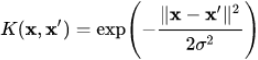 
dataset.shape(instaces, features)-->

X1D = np.linspace(-4, 4, 9).reshape(-1, 1) #X1D=array([ [-4.],[-3.],[-2.],[-1.],[ 0.],[ 1.],[ 2.],[ 3.],[ 4.] ])
x1_example=X1D[3,0] #x1_example=-1.0
gamma=0.3

def gaussian_rbf(x, landmark, gamma):     # arry_like #ord default=L2 norm
    return np.exp(-gamma * np.linalg.norm(x-landmark, axis=1)**2) #x offset landmark positions to the left

for landmark in (-2,1):
    k = gaussian_rbf( np.array([ [x1_example] ]), np.array([ [landmark] ]), gamma)
    print( "Phi({}, {}) = {}".format(x1_example, landmark, k) )

It is a bell-shaped function varying from 0 (very far away from the landmark) to 1 (at the landmark). Now we are ready to compute the new features. For example, let's look at the instance x1 = –1: it is located at a distance of 1 from the first landmark(1=-2), and 2 from the second landmark(1=1). Therefore its new features are  ≈ 0.74 and ≈ 0.30. The plot on the right of Figure 5-8 shows the transformed dataset (dropping the original features). As you can see, it is now linearly separable.

def gaussian_rbf(x, landmark, gamma):     # arry_like #ord default=L2 norm
    return np.exp(-gamma * np.linalg.norm(x-landmark, axis=1)**2)
    #if x =array( [[-4.5],...,[4.5]] )
    # x-landmark=x+2= array( [[-2.5],...,[6.5] ) # axis=1 means the operation on row
    # np.linalg.norm(x-landmark, axis=1)=np.linalg.norm(x1s+2, axis=1,ord=2,keepdims=False) #1D
    #note: np.linalg.norm(x1s+2, axis=1,ord=2,keepdims=False)==np.linalg.norm(x1s+2, axis=1,ord=1,keepdims=False)
    #since each row only has one column with 1 element
    # np.linalg.norm(x-landmark, axis=1)=np.ravel(np.absolute(x1s))
    
gamma=0.3

x1s = np.linspace(-4.5, 4.5, 200).reshape(-1, 1) #2D array[[-4.5],...,[4.5]]
x2s = gaussian_rbf(x1s,-2,gamma) #using RBF(x, x'=-2) for x_axis
x3s = gaussian_rbf(x1s,1,gamma)  #using RBF(x, x'=1) for x_asis

X1D = np.linspace(-4, 4, 9).reshape(-1, 1)
            #using RBF(X1D, x'=-2) as x2    #using RBF(X1D, x'=1) as x3
XK = np.c_[ gaussian_rbf(X1D, -2, gamma), gaussian_rbf(X1D, 1, gamma) ]
yk = np.array([0, 0, 1, 1, 1, 1, 1, 0, 0])

plt.figure( figsize=(10.5, 4) )

plt.subplot(121)
plt.grid(True, which="both")
plt.axhline(y=0, color="k") #x-coordinate
plt.scatter(x=[-2,1], y=[0,0], s=150, alpha=0.5, c="red") # landmark or where Gaussian RBF to center at
         #x                #y
plt.plot(X1D[:,0][yk==0], np.zeros(4), "bs") #label
plt.plot(X1D[:,0][yk==1], np.zeros(5), "g^")
plt.plot(x1s, x2s, "g--") #x2s = gaussian_rbf(x1s,-2,gamma)
plt.plot(x1s, x3s, "b:") #x3s = gaussian_rbf(x1s,1,gamma)
plt.gca().get_yaxis().set_ticks([0, 0.25, 0.5, 0.75, 1])
plt.xlabel(r"$x_1$", fontsize=20)
plt.ylabel(r"Similarity", fontsize=14)
plt.annotate(r"$\mathbf{x}$",  # \mathbf{}  #math bracket for {}
             xy=(X1D[3,0],0),  #select a datapoint(an instance) as input then use twice gaussian_rbf for prediction
             xytext=(-0.5, 0.2),
             ha="center",
             arrowprops=dict(facecolor="black", shrink=0.1),
             fontsize=18,
            )
plt.text(-2, 0.9, "$x_2$", ha="center", fontsize=20)
plt.text(1, 0.9, "$x_3$", ha="center", fontsize=20)
plt.axis([-4.5, 4.5, -0.1, 1.1])

plt.subplot(122)
plt.grid(True, which="both")
plt.axhline(y=0, color="k")
plt.axvline(x=0, color="k")
plt.plot(XK[:,0][yk==0], XK[:,1][yk==0], "bs") #(RBF_x2,RBF_x3), yk==0
plt.plot(XK[:,0][yk==1], XK[:,1][yk==1], "g^") #(RBF_x2,RBF_x3), yk==1
plt.xlabel(r"$x_2$", fontsize=20)
plt.ylabel(r"$x_3$   ", fontsize=20, rotation=0)
plt.annotate(r'$\phi\left(\mathbf{x}\right)$',
             xy=(XK[3,0], XK[3,1]),#the datapoint we selected previously and did twice gaussian_rbf for prediction
             xytext=(0.65,0.50),
             ha="center",
             arrowprops=dict(facecolor="black", shrink=0.1),
             fontsize=18,
            ) # \left( ="("  # \right( =")"
plt.plot([-0.1,1.1], [0.57,-0.1], "r--", linewidth=3) #decision boundary #seperating hyperplane
plt.axis([-0.1, 1.1, -0.1, 1.1])

plt.subplots_adjust(right=1)
plt.show()

summary: assuming you drop the original features
dataset ==>Two k(dataset_X, landmark_X')= ==>new dataset(exponential value, exponential value ) which is linearly separable.

assuming you not drop the original features https://blog.csdn.net/Linli522362242/article/details/104151351

dataset ==> One k(dataset_X,landmark_X')=assuming y=x**2==>new datset(dataset_X, X**2) which is linearly separable.

You may wonder how to select the landmarks. The simplest approach is to create a landmark at the location of each and every instance in the dataset. This creates many dimensions and thus increases the chances that the transformed training set will be linearly separable. The downside is that a training set with m instances and n features gets transformed into a training set with m instances and m features (assuming you drop the original features). If your training set is very large, you end up with an equally large number of features.

Gaussian RBF Kernel

Just like the polynomial features method, the similarity features method can be useful with any Machine Learning algorithm, but it may be computationally expensive to compute all the additional features, especially on large training sets. However, once again the kernel trick does its SVM magic: it makes it possible to obtain a similar result as if you had added many similarity features, without actually having to add them. Let’s try the Gaussian RBF kernel using the SVC class:

rbf_kernel_svm_clf = Pipeline([
    ("scaler", StandardScaler() ),
    ("svm_clf", SVC(kernel="rbf", gamma=5, C=0.001) )
])

rbf_kernel_svm_clf.fit(X,y)

This model is represented on the bottom left of Figure 5-9. The other plots show models trained with different values of hyperparameters gamma (γ) and C. Increasing gamma(γ) makes the bell-shape curve narrower (see the left plot of Figure 5-8), and as a result each instance’s range of influence is smaller: the decision boundary ends up being more irregular, wiggling扭动 around individual instances. Conversely, a small gamma(γ) value makes the bell-shaped curve wider, so instances have a larger range of influence, and the decision boundary ends up smoother. So γ acts like a regularization hyperparameter: if your model is overfitting, you should reduce it, and if it is underfitting, you should increase it (similar to the C hyperparameter).

from sklearn.svm import SVC

gamma1, gamma2 = 0.1, 5
C1, C2 = 0.001,1000
hyperparams = (gamma1, C1), (gamma1, C2), (gamma2, C1), (gamma2,C2)

svm_clfs = []
for gamma, C in hyperparams:
    rbf_kernel_svm_clf = Pipeline([
        ("scaler", StandardScaler()),
        ("svm_clf", SVC(kernel="rbf", gamma=gamma, C=C))
    ])
    rbf_kernel_svm_clf.fit(X,y)
    svm_clfs.append(rbf_kernel_svm_clf)

def plot_predictions(clf, axes):
    x0s = np.linspace(axes[0], axes[1], 100)
    x1s = np.linspace(axes[2], axes[3], 100)
    x0, x1 = np.meshgrid(x0s, x1s)
    X = np.c_[x0.ravel(), x1.ravel()]
    y_pred = clf.predict(X).reshape(x0.shape)
    y_decision = clf.decision_function(X).reshape(x0.shape) #decision broundary
    plt.contourf(x0,x1, y_pred, cmap=plt.cm.brg, alpha=0.2)
    plt.contourf(x0,x1,y_decision,cmap=plt.cm.brg, alpha=0.1)    

def plot_dataset(X,y, axes):
    plt.plot(X[:,0][y==0], X[:,1][y==0], "bs")
    plt.plot(X[:,0][y==1], X[:,1][y==1], "g^")
    plt.axis(axes)
    plt.grid(True, which="both")
    plt.xlabel(r"$x_1$", fontsize=20)
    plt.ylabel(r"$x_2$", fontsize=20, rotation=0)    
    
fig, axes = plt.subplots(nrows=2, ncols=2, figsize=(10.5,7))

for i,svm_clf in enumerate(svm_clfs):
    plt.sca( axes[i//2, i%2] )###
    plot_predictions(svm_clf, [-1.5,2.5, -1,1.5])
    plot_dataset(X,y, [-1.5,2.5, -1,1.5])
    gamma, C=hyperparams[i]
    plt.title( r"$\gamma = {},C={}$".format(gamma, C), fontsize=16 )

plt.subplots_adjust(hspace=0.4)    
plt.show()

Figure 5-9. SVM classifiers using an RBF kernel
Other kernels exist but are used much more rarely. For example, some kernels are specialized for specific data structures. String kernels are sometimes used when classifying text documents or DNA sequences (e.g., using the string subsequence kernel or kernels based on the Levenshtein distance).
###########################################
TIP
With so many kernels to choose from, how can you decide which one to use? As a rule of thumb, you should always try the linear kernel first (remember that LinearSVC is much faster than SVC(kernel="linear")), especially if the training set is very large or if it has plenty of features. If the training set is not too large, you should try the Gaussian RBF kernel as well; it works well in most cases. Then if you have spare time and computing power, you can also experiment with a few other kernels using crossvalidation and grid search, especially if there are kernels specialized for your training set’s data structure.
###########################################

Computational Complexity

The LinearSVC class is based on the liblinear library, which implements an optimized algorithm for linear SVMs. It does not support the kernel trick, but it scales almost linearly with the number of training instances and the number of features: its training time complexity is roughly O(m × n).

The algorithm takes longer if you require a very high precision. This is controlled by the tolerance hyperparameter ϵ (called tol in Scikit-Learn). In most classification tasks, the default tolerance is fine. 

The SVC class is based on the libsvm library, which implements an algorithm that supports the kernel trick. The training time complexity is usually between O( × n) and O( × n). Unfortunately, this means that it gets dreadfully slow when the number of training instances gets large (e.g., hundreds of thousands of instances). This algorithm is perfect for complex but small or medium training sets. However, it scales缩放 well with the number of features, especially with sparse features (i.e., when each instance has few nonzero features). In this case, the algorithm scales roughly with the
average number of nonzero features per instance. Table 5-1 compares Scikit-Learn’s SVM classification classes.

SVM Regression

As we mentioned earlier, the SVM algorithm is quite versatile多用途的: not only does it support linear and nonlinear classification, but it also supports linear and nonlinear regression. The trick is to reverse the objective: instead of trying to fit the largest possible street(margin) between two classes while limiting margin violations, SVM Regression tries to fit as many instances as possible on the street while limiting margin violations (i.e., instances off the street). The width of the street is controlled by a hyperparameter ϵ(Epsilon). Figure 5-10 shows two linear SVM Regression models trained on some random linear data, one with a large margin (ϵ = 1.5) and the other with a small margin (ϵ = 0.5).

Maximum Margin Classifiers 

linear models： OR 

this function margin is calculated by label*(+b)   

to solve 
-->At first, solve  to find the points(some of them wil be the support vectors) with the smallest margin, then we must maximize that margin .

since the constraints  , so the minimum value is 1 which is controlled by the support vectors(find them at first);  Then maximize  ==> maximize ==> is equivalent to minimizing ==> 

  1 is the minimum margin size and in which the slack variables are constrained to satisfy . Points for which  lie inside the margin, but on the correct side of the decision boundary, and those data points for which ξn > 1 lie on the wrong side of the decision boundary and are misclassified.

SVM Regression tries to fit as many instances as possible on the street while limiting margin violations (i.e., instances off the street/margin), so we should take care of  and The width of the street is controlled by a hyperparameter ϵ(Epsilon)

Our goal is now to maximize the margin while softly penalizing points that lie on the wrong side of the margin boundary. We therefore minimize             
where the parameter C > 0 controls the trade-off between the slack variable penalty and the margin. Because any point that is misclassified has ξn > 1, it follows that  is an upper bound on the number of misclassified points. The parameter C is therefore analogous相似的 to (the inverse of) a regularization coefficient because it controls the trade-off between minimizing training errors and controlling model complexity. In the limit C → ∞, we will recover the earlier support vector machine for separable data.
################################

By increasing the value of the hyperparameter  (regularization coefficient), we increase the regularization strength(for tackling the problem of overfitting) and shrink the weights of our model(or reduce the value of wj or bj) since we want to make the function attain the minimum( including )
################################
a smaller C value leads to a wider street but more margin violations（too many ξn OR  too large, Note: we want to minimize the cost function）
a high C value the classifier makes fewer margin violations but ends up with a smaller margin

svm_reg1 = LinearSVR(epsilon=1.5, random_state=42)
svm_reg2 = LinearSVR(epsilon=0.5, random_state=42)
svm_reg1.fit(X,y)
svm_reg2.fit(X,y)

def find_support_vectors(svm_reg, X, y):
    y_pred = svm_reg.predict(X)
    off_margin = ( np.abs(y-y_pred)>=svm_reg.epsilon )
    return np.argwhere(off_margin)

svm_reg1.support_ = find_support_vectors(svm_reg1, X,y)
svm_reg2.support_ = find_support_vectors(svm_reg2, X,y)

eps_x1 = 1
eps_y_pred = svm_reg1.predict([ [eps_x1] ])

def plot_svm_regression(svm_reg, X, y, axes):
    x1s = np.linspace(axes[0], axes[1], 100).reshape(100,1) #axes[0]......axes[1]
    y_pred = svm_reg.predict(x1s)
    plt.plot(x1s, y_pred, "k-", linewidth=2, label=r"$\hat{y}$") #decision boundary
    plt.plot(x1s, y_pred + svm_reg.epsilon, "k--") # margin
    plt.plot(x1s, y_pred - svm_reg.epsilon, "k--") # margin
    plt.scatter( X[svm_reg.support_], y[svm_reg.support_], s=180, facecolors="#FFAAAA" )#np.abs(y-y_pred)>=svm_reg.epsilon
    plt.plot(X,y, "bo")
    plt.xlabel(r"$x_1$", fontsize=18)
    plt.legend(loc="upper left", fontsize=18)
    plt.axis(axes)
               
fig, axes = plt.subplots(ncols=2, figsize=(9,4), sharey=False)
               
plt.sca(axes[0])
plot_svm_regression( svm_reg1, X,y, [0,2, 3,11] )
plt.title(r"$\epsilon={}$".format(svm_reg1.epsilon), fontsize=18)
plt.ylabel(r"$y$", fontsize=18, rotation=0)
plt.annotate(
    '',
    xy=(eps_x1, eps_y_pred),
    xycoords="data",
    xytext=(eps_x1, eps_y_pred-svm_reg1.epsilon),
    textcoords="data",
    arrowprops={'arrowstyle':"<->", 'linewidth':1.5}
)
plt.text(0.91, 5.6, r"$\epsilon$", fontsize=20)
               
plt.sca(axes[1])
plot_svm_regression(svm_reg2, X,y, [0,2, 3,11])
plt.title(r"$\epsilon={}$".format(svm_reg2.epsilon), fontsize=18)
plt.ylabel(r"$y$", fontsize=18, rotation=0)

plt.show()

Figure 5-10. SVM Regression

Adding more training instances within the margin does not affect the model's predictions; thus, the model is said to be ϵ-insensitive.

You can use Scikit-Learn's LinearSVR class to perform linear SVM Regression. The following code produces the model represented on the left of Figure 5-10 (the training data should be scaled and centered first):

np.random.seed(42)
m=50
X = 2*np.random.rand(m,1)
y = (4+3*X + np.random.randn(m,1)).ravel()

from sklearn.svm import LinearSVR

svm_reg = LinearSVR(epsilon=1.5, random_state=42)
svm_reg.fit(X,y)

 
###########################extra materials

################################

By increasing the value of the hyperparameter  (regularization coefficient), we increase the regularization strength(for tackling the problem of overfitting) and shrink the weights of our model(or reduce the value of wj or bj) since we want to make the function attain the minimum( including )
################################

minimize the cost function

minimize;      larger, large regularization strength(shrink the weights)

where the parameter C > 0 controls the trade-off between the slack variable penalty and the margin. Because any point that is misclassified has ξn > 1, it follows that  is an upper bound on the number of misclassified points. The parameter C is therefore analogous相似的 to (the inverse of) a regularization coefficient because it controls the trade-off between minimizing training errors and controlling model complexity. In the limit C → ∞, we will recover the earlier support vector machine for separable data.
SVM Regression tries to fit as many instances as possible on the street while limiting margin violations (i.e., instances off the street/margin), so we should take care of  and The width of the street is controlled by a hyperparameter ϵ(Epsilon); but now , larger C, larger , reduce the influence from , then regularization strength is decreased.
###########################

To tackle nonlinear regression tasks, you can use a kernelized SVM model. For example, Figure 5-11 shows SVM Regression on a random quadratic training set, using a 2nd-degree polynomial kernel. There is little regularization on the left plot (i.e., a large C value: Adding more training instances within the margin), and much more regularization on the right plot (i.e., a small C value).

from sklearn.svm import SVR

svm_poly_reg1 = SVR(kernel="poly", degree=2, C=1000, epsilon=0.1, gamma="scale")
svm_poly_reg2 = SVR(kernel="poly", degree=2, C=0.001, epsilon=0.1, gamma="scale")
svm_poly_reg1.fit(X,y)
svm_poly_reg2.fit(X,y)

fig, axes = plt.subplots(ncols=2, figsize=(9,4), sharey=False)

plt.sca(axes[0])
plot_svm_regression(svm_poly_reg1, X,y, [-1,1, 0,1])
plt.title(r"$degree={}, C={}, \epsilon={}$".format(svm_poly_reg1.degree, svm_poly_reg1.C, svm_poly_reg1.epsilon),
          fontsize=18
         )
plt.ylabel(r"$y$", fontsize=18, rotation=0)

plt.sca(axes[1])
plot_svm_regression(svm_poly_reg2, X,y, [-1,1, 0,1])
plt.title(r"$degree={}, C={}, \epsilon={}$".format(svm_poly_reg2.degree, svm_poly_reg2.C, svm_poly_reg2.epsilon),
          fontsize=18
         )
plt.ylabel(r"$y$", fontsize=18, rotation=0)

plt.show()

Figure 5-11. SVM regression using a 2nd-degree polynomial kernel

The following code produces the model represented on the left of Figure 5-11 using Scikit-Learn’s SVR class (which supports the kernel trick). The SVR class is the regression equivalent of the SVC class, and the LinearSVR class is the regression equivalent of the LinearSVC class. The LinearSVR class scales linearly with the size of the training set (just like the LinearSVC class), while the SVR class gets much too slow when the training set grows large (just like the SVC class).

from sklearn.svm import SVR

svm_poly_reg = SVR(kernel="poly", degree=2, C=100, epsilon=0.1, gamma="scale")
svm_poly_reg.fit(X,y)

#######################
NOTE

SVMs can also be used for outlier detection; see Scikit-Learn’s documentation for more details.
#######################

Under the Hood

This section explains how SVMs make predictions and how their training algorithms work, starting with linear SVM classifiers. You can safely skip it and go straight to the exercises at the end of this chapter if you are just getting started with Machine Learning, and come back later when you want to get a deeper understanding of SVMs.

First, a word about notations: in https://blog.csdn.net/Linli522362242/article/details/104005906 we used the convention of putting all the model parameters in one vector θ, including the bias term and the input feature weights to , and adding a bias input x0 = 1 to all instances. In this chapter, we will use a different convention, which is more convenient (and more common) when you are dealing with SVMs: the bias term will be called b and the feature weights vector
will be called w. No bias feature will be added to the input feature vectors.

Decision Function and Predictions

The linear SVM classifier model predicts the class of a new instance x by simply computing the decision function : if the result is positive, the predicted class ŷ is the positive class (1), or else it is the negative class (0); see Equation 5-2.

Equation 5-2. Linear SVM classifier prediction 
https://blog.csdn.net/Linli522362242/article/details/104151351

Figure 5-12 shows the decision function that corresponds to the model on the right of Figure 5-4 : it is a two-dimensional plane since this dataset has two features (petal width and petal length). The decision boundary is the set of points where the decision function is equal to 0: it is the intersection of two planes, which is a straight line (represented by the thick solid line).
The dashed lines represent the points where the decision function is equal to 1 or –1: they are parallel and at equal distance to the decision boundary, forming a margin around it. Training a linear SVM classifier means finding the value of w and b that make this margin as wide as possible while avoiding margin violations (hard margin: strictly impose that all instances be off the street/margin and on the right side) or limiting them (soft margin: The objective is to find a good balance between keeping the street as large as possible and limiting the margin violations (i.e., instances that end up in the middle of the street or even on the wrong side)).

iris = datasets.load_iris()
X = iris["data"][:, (2,3)] # petal length, petal width
y = (iris["target"]==2).astype(np.float64) # Iris virginica
y

scaler = StandardScaler()
svm_clf2 = LinearSVC( C=100, loss="hinge", random_state=42 )

scaled_svm_clf2 = Pipeline([
    ("scaler", scaler),
    ("linear_svc", svm_clf2),
])

scaled_svm_clf2.fit(X,y)

#As we known as that after doing StandardScaler() then doing linear_svc, the 
#new hyperplane has been Offset (the original without doing StandardScaler() prior to linear_svc); 
#and here we want to use original dataset so we have to do following processes
 
#Convert to unscaled parameters
#the seperating hyperplane wx+b
#the seperating hyperplane wx+b=0 means the distance of the points on the seperating
#hyperplane to the seperating hyperplane is equal to 0
 
#After doing StandardScare,the seperating hyperplane wx+b=0 --offset-->
# w*(x-mean)/scale+b=0 --> w*x/scale +b- w*mean/scale =0
# new w1=w/scale, new b1=b-w*mean/scale
 
#note: the original decision_function: wx+b
#      the new decision_function: w*(x-mean)/scale+b offset (-mean)/scale
 
#decision_function: represents the distance from the parameter instance(including some data points) to the separating hyperplane represented by each class
#-scaler.mean_/scaler.scale_ to offset the original separating hyperplane of datapoints
b2 = svm_clf2.decision_function([ -scaler.mean_/scaler.scale_ ])
w2 = svm_clf2.coef_[0] / scaler.scale_
svm_clf2.intercept_ = np.array([b2]) #######new intercept
svm_clf2.coef_ = np.array([w2])      #######new coefficients

from mpl_toolkits.mplot3d import Axes3D
                                        #Petal length    #Petal width 
def plot_3D_decision_function(ax, w, b, x1_lim=[4,6], x2_lim=[0.8,2.8]):
    x1_in_bounds = ( X[:,0]>x1_lim[0]) & (X[:,0]<x1_lim[1] ) #Petal length 
    X_crop = X[x1_in_bounds] #select data
    y_crop = y[x1_in_bounds]
    x1s = np.linspace(x1_lim[0], x1_lim[1], 20)
    x2s = np.linspace(x2_lim[0], x2_lim[1], 20)
    x1,x2 = np.meshgrid(x1s, x2s)
    xs = np.c_[x1.ravel(), x2.ravel()]
    df = (xs.dot(w) + b).reshape(x1.shape) # w^x+b
    m = 1 / np.linalg.norm(w) #??
    #separating hyperplane: w0*x1s + w1*x2s +b=0 ==> x2s = -x1s*w0/w1 - b/w1
    boundary_x2s = -x1s*(w[0]/w[1]) - b/w[1]
    #upper-support hyperplane: w0*x1s + w1*x2s +b=1 ==> x2s = x1s*w0/w1 - (b-1)/w1
    margin_x2s_1 = -x1s*(w[0]/w[1]) - (b-1)/w[1]
    #lower-suppert hyperplane: w0*x0 + w1*x1 + b=-1 ==> x2s = x1s*w0/w1 - (b+1)/w1
    margin_x2s_2 = -x1s*(w[0]/w[1]) - (b+1)/w[1]

                        #x2.shape=(20, 20)
    ax.plot_surface(x1s, x2, np.zeros_like(x1), color="b", alpha=0.2, cstride=100, rstride=100)
    ax.plot(X_crop[:,0][y_crop==1], X_crop[:,1][y_crop==1], 0, "g^")
    ax.plot(X_crop[:,0][y_crop==0], X_crop[:,1][y_crop==0], 0, "bs")
    ax.plot_wireframe(x1, x2, df, alpha=0.3, color="k") ##########
    ax.plot(x1s, boundary_x2s, 0, "k-", linewidth=2, label=r"$h=0$") #z=0
    ax.plot(x1s, margin_x2s_1, 0, "k--", linewidth=2, label=r"$h=\pm 1$") #z=0
    ax.plot(x1s, margin_x2s_2, 0, "k--", linewidth=2)
    ax.axis(x1_lim + x2_lim)
    ax.text(4.5, 2.5, 3.8, "Decision function $h$", fontsize=16)
    ax.set_xlabel(r"Petal length", fontsize=16, labelpad=10)
    ax.set_ylabel(r"Petal width", fontsize=16, labelpad=10)
    ax.set_zlabel(r"$h=\mathbf{w}^T \mathbf{x} + b$", fontsize=18, labelpad=5)
    ax.legend(loc="upper left", fontsize=16)
    
fig = plt.figure(figsize=(13,8))
ax1 = fig.add_subplot(111, projection="3d")
plot_3D_decision_function(ax1, w=svm_clf2.coef_[0], b=svm_clf2.intercept_[0])

Figure 5-12. Decision function for the iris dataset

Training Objective

Consider the slope of the decision function: it is equal to the norm of the weight vector, ∥ w ∥. If we divide this slope by 2, the points where the decision function is equal to ±1 are going to be twice as far away from the decision boundary. In other words, dividing the slope by 2 will multiply the margin by 2. Perhaps this is easier to visualize
in 2D in Figure 5-13. The smaller the weight vector w, the larger the margin.

def plot_2D_decision_function(w,b, ylabel=True, x1_lim=[-3,3]):
    x1 = np.linspace(x1_lim[0], x1_lim[1], 200)
    y = w*x1+b
    m = 1/w # y=w*x1+b=1 ==> x1=(1-b)/w
            # y=w*x1+b=-1 ==> x1=(1+b)/w
    plt.plot(x1,y, label="y=wx+b=0")    #y =w*x1+b = 0
    plt.plot(x1,y+1, label="y=wx+b=1") #y =w*x1+b =1
    plt.plot(x1,y-1, label="y=wx+b=-1") #y =w*x1+b =-1
    plt.plot(x1_lim, [1,1], "k:")
    plt.plot(x1_lim, [-1,-1], "k:")
    plt.axhline(y=0, color="k")
    plt.axvline(x=0, color="k")
    plt.plot([m,m],[0,1], "b")
    plt.plot([-m,-m],[0,-1], "b")
    plt.plot([-m,m], [0,0],"k-o", linewidth=3)
    plt.axis(x1_lim + [-2,2])
    plt.xlabel(r"$x_1$", fontsize=16)
    if ylabel:
        plt.ylabel(r"$w_1 x_1$   ", rotation=0, fontsize=16)
    plt.legend(loc="upper left")
    plt.title(r"$w_1={}$".format(w), fontsize=16)

plt.figure(figsize=(12, 3.2))

plt.subplot(121)
plot_2D_decision_function(1,0)

plt.subplot(122)
plot_2D_decision_function(0.5,0,ylabel=False)

plt.show()

Figure 5-13. A smaller weight vector results in a larger margin

So we want to minimize ∥ w ∥ to get a large margin. However, if we also want to avoid any margin violation (hard margin), then we need the decision function( + b) to be greater than 1 for all positive training instances, and lower than –1 for negative training instances. If we define label  = –1 for negative instances (if = 0) and = 1 for positive instances (if = 1), then we can express this constraint as ( + b) ≥ 1 for all instances.

We can therefore express the hard margin linear SVM classifier objective as the constrained optimization problem in Equation 5-3.

Equation 5-3. Hard margin linear SVM classifier objective 
###########################################
We are minimizing , which is equal to , rather than minimizing ∥ w ∥. This is because it will give the same result (since the values of w and b that minimize a value also minimize half of its square), but has a nice and simple derivative (it is just w) while ∥ w ∥ is not differentiable at w = 0. Optimization algorithms work much better on differentiable functions.
###########################################

To get the soft margin objective, we need to introduce a slack variable ≥ 0 for each instance:  measures how much the instance is allowed to violate the margin. We now have two conflicting objectives: making the slack variables as small as possible to reduce the margin violations, and making as small as possible to increase the margin. This is where the C hyperparameter comes in: it allows us to define the trade‐off between these two objectives. This gives us the constrained optimization problem in Equation 5-4.

Equation 5-4. Soft margin linear SVM classifier objective    

Minimize, ;  Constraints: , 
Put the constraints together to construct the corresponding Lagrangian

  a = 
where {} and {} are Lagrange multipliers. The corresponding set of KKT conditions are given by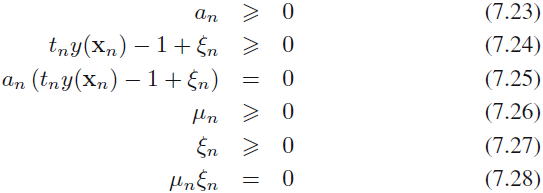

where n = 1, . . . , N.
https://blog.csdn.net/Linli522362242/article/details/104151351

The hard margin(without slacks variables)

 a =  the constraints 
Quadratic Programming

The hard margin and soft margin problems are both convex quadratic optimization problems with linear constraints. Such problems are known as Quadratic Programming二次规划 (QP) problems. Many off-the-shelf solvers are available to solve QP problems using a variety of techniques The general problem formulation is given by Equation 5-5.

Equation 5-5. Quadratic Programming problem #p is a vertical vector

Note that the expression A · p ≤ b actually defines constraints: for i =1, 2, ⋯, , where is the vector containing the elements of the row of A and is the element of b.

You can easily verify that if you set the QP parameters in the following way, you get the hard margin linear SVM classifier objective:
• = n + 1, where n is the number of features (the +1 is for the bias term).
• = m, where m is the number of training instances.  (A is bias(0th column is all 0s)+training dataset  )
• H is the × identity matrix , except with a zero in the top-left cell (to ignore the bias term(0th column is all 0s)).  so ==
• f = 0, an -dimensional vector full of 0s.  in to ignore the bias term
• b = 1, an -dimensional vector full of 1s. so all ==1
•, where  is equal to with an extra bias feature = 1. 
 * == 1==

So one way to train a hard margin linear SVM classifier is just to use an off-the-shelf QP solver by passing it the preceding parameters. The resulting vector p will contain the bias term b = p0 and the feature weights . Similarly, you can use a QP solver to solve the soft margin problem.

However, to use the kernel trick we are going to look at a different constrained optimization problem
########################## extra
https://blog.csdn.net/qcyfred/article/details/71598807

Hessian矩阵

https://optimization.mccormick.northwestern.edu/index.php/Quadratic_programming

Note the correct 2-degree gradient matrix [ [6 2], [2,2] ], here just for convenient computation  [ [6 2], [2,1] ]
##########################

The Dual Problem对偶问题

Given a constrained optimization problem, known as the primal problem原始问题, it is possible to express a different but closely related problem, called its dual problem. The solution to the dual problem typically gives a lower bound to the solution of the primal problem, but under some conditions it can even have the same solutions as the primal problem. Luckily, the SVM problem happens to meet these conditions, so you can choose to solve the primal problem or the dual problem; both will have the same solution. Equation 5-6 shows the dual form of the linear SVM objective (if you are interested in knowing how to derive the dual problem from the primal problem see https://blog.csdn.net/Linli522362242/article/details/104151351）.

Equation 5-6. Dual form of the linear SVM objective (maximize margin classifier)

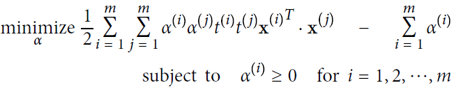 OR 

Once you find the vector that minimizes this equation (using a QP solver), you can compute  and that minimize the primal problem by using Equation 5-7.


Equation 5-7. From the dual solution to the primal solution 

The dual problem is faster to solve than the primal when the number of training instances is smaller than the number of features. More importantly, it makes the kernel trick possible, while the primal does not. So what is this kernel trick anyway?

Kernelized SVM

Suppose you want to apply a 2nd-degree polynomial transformation to a two dimensional training set (such as the moons training set), then train a linear SVM classifier on the transformed training set. Equation 5-8 shows the 2nd-degree polynomial mapping function ϕ that you want to apply.

Equation 5-8. Second-degree polynomial mapping 
two-dimensional input space x =

Notice that the transformed vector is three-dimensional instead of two-dimensional. Now let's look at what happens to a couple of two-dimensional vectors, a and b, if we apply this 2nd-degree polynomial mapping and then compute the dot product of the transformed vectors (See Equation 5-9).

Equation 5-9. Kernel trick for a 2nd-degree polynomial mapping 
How about that? The dot product of the transformed vectors is equal to the square of the dot product of the original vectors: .

Now here is the key insight: if you apply the transformation ϕ to all training instances, then the dual problem (see Equation 5-6) will contain the dot product .
######################################## extra

####################

The hard margin(without slacks variables)

 a =  the constraints 

 

SVM Regression tries to fit as many instances as possible on the street while limiting margin violations
(i.e., instances off the street).

Now here is the key insight: if you apply the transformation ϕ to all training instances, then the dual problem (see Equation 5-6) will contain the dot product .     #### seee equation 6.6
But if ϕ is the 2nd-degree polynomial transformation defined in Equation 5-8, then you can replace this dot product of transformed vectors simply by . So you don't actually need to transform the training instances at all (###you just use the instances a and b instead of all instances): just replace the dot product by its square in Equation 5-6. The result will be strictly the same as if you went through the trouble of actually transforming the training set then fitting a linear SVM algorithm(do   then  find the corresponding the mapped feature space ϕ, and finally do compute the dot product , Note we not do prediction here and we need the instances'  mapped feature space), but this trick makes the whole process much more computationally efficient. This is the essence of the kernel trick.

The function is called a 2nd-degree polynomial kernel. In Machine Learning, a kernel is a function capable of computing the dot product based only on the original vectors a and b, without having to compute (or even to know about) the transformation ϕ. Equation 5-10 lists some of the most commonly used kernels.

 
##################################
Mercer's Theorem
According to Mercer's theorem, if a function K(a, b) respects a few mathematical conditions called Mercer's conditions (K must be continuous, symmetric in its arguments so , etc.), then there exists a function ϕ that maps a and b into another space (possibly with much higher dimensions) such that. So you can use K as a kernel since you know ϕ exists, even if you don't know what ϕ is. In the case of the Gaussian RBF kernel, it can be shown that ϕ actually maps each training instance to an infinite-dimensional space, so it's a good thing you don’t need to actually perform the mapping!

Note that some frequently used kernels (such as the Sigmoid kernel) don't respect不满足 all of Mercer’s conditions, yet they generally work well in practice.
##################################

05_Support Vector Machines_03
https://blog.csdn.net/Linli522362242/article/details/104403372