05_Support Vector Machines_hinge_support vectors_decision function_Lagrange multiplier拉格朗日乘数
https://blog.csdn.net/Linli522362242/article/details/104151351
05_Support Vector Machines_02_Polynomial Kernel_Gaussian RBF_Kernelized SVM Regression_Quadratic Problem
https://blog.csdn.net/Linli522362242/article/details/104280075
If we strictly impose that all instances be off the street and on the right side, this is called hard margin classification.
linear models: ![]() OR
OR ![]()
where ![]() denotes a fixed feature-space transformation, and we have made the bias parameter b explicit.
denotes a fixed feature-space transformation, and we have made the bias parameter b explicit.

Figure 7.1 The margin is defined as the perpendicular distance
(https://blog.csdn.net/Linli522362242/article/details/104151351 ![]() ) between the decision boundary and the closest of the data points, as shown on the left figure. (we wish to optimize the parameters w and b in order to) Maximizing the margin leads to a particular choice of decision boundary, as shown on the right. The location of this boundary is determined by a subset of the data points, known as support vectors, which are indicated by the circles.
) between the decision boundary and the closest of the data points, as shown on the left figure. (we wish to optimize the parameters w and b in order to) Maximizing the margin leads to a particular choice of decision boundary, as shown on the right. The location of this boundary is determined by a subset of the data points, known as support vectors, which are indicated by the circles.
to solve 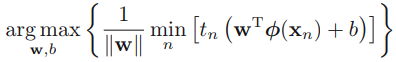
-->At first,  (to find the closest of data points to decision boundary) ,
-->Next, maximize ![]() for maximizing the margin( to choose the decision boundary or to find the support vectors that determine the location boundary) ==> maximize
for maximizing the margin( to choose the decision boundary or to find the support vectors that determine the location boundary) ==> maximize ![]() ==> is equivalent to minimizing
==> is equivalent to minimizing ![]() ==>
==> ![]() s.t.
s.t. ![]()
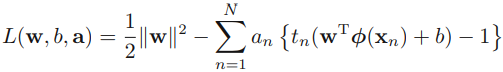
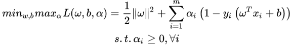
In order to solve this constrained optimization (maximize margin) problem, we introduce Lagrange multipliers拉格朗日乘数 ![]() 0, with one multiplier
0, with one multiplier  for each of the constraints, giving the Lagrangian function
#######################
minimize ![]() s.t.
s.t. ![]() ==> maximize:
==> maximize: 
 ????
????
Let's do ![]() s.t.
s.t. ![]() ==>
==> 
#0. ![]() =1, OR
=1, OR ![]() =0,
=0,
no matter how ![]() changes, the
changes, the ![]() must be 0
must be 0
the left equation ![]() is always equivalent to the right equation , inside the feasible solution area. but we require
is always equivalent to the right equation , inside the feasible solution area. but we require ![]() >0, since Any data point for which
>0, since Any data point for which ![]() = 0 will not appear in the sum in (7.13
= 0 will not appear in the sum in (7.13 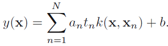 ) and hence plays no role in making predictions for new data points.
#1. ![]() >1,
>1, ![]() >0
>0
if ![]() =0 then the left equation
=0 then the left equation ![]() is equivalent to , but we need to drop it, the reason see above(#0.).
is equivalent to , but we need to drop it, the reason see above(#0.).
if ![]() >0 then the left equation
>0 then the left equation ![]() is not equivalent to
is not equivalent to
then ![]() -->
--> ![]() ,
,  --> -
--> -![]() , so we need to maximize
, so we need to maximize ![]() to let the right equation
to let the right equation ![]() is equivalent/close to the left equation
is equivalent/close to the left equation ![]()
![]() ==>
==>![]() + maximize
+ maximize
#3. minimize ![]() s.t.
s.t. ![]() ==> minimize{
==> minimize{ ![]() + maximize }
+ maximize }
==> ==>When the Slater theorem is satisfied and the process meets the KKT condition, the original problem is transformed into a dual problem==>(dual problem)
since ![]() is a label (+1 or -1), b is a constant,
is a label (+1 or -1), b is a constant, ![]() is a input instance(constant), then we need to maximize w for maximizing
is a input instance(constant), then we need to maximize w for maximizing ![]() ==> to maximize
==> to maximize ![]() (
(![]() >0); In other words,
>0); In other words, ![]() constrols the influence from the changes of
constrols the influence from the changes of ![]()
==> maximize: ![]()
#######################
###we put the constraints together
where a = ![]() . Note the minus sign in front of the Lagrange multiplier term, because we are minimizing (
. Note the minus sign in front of the Lagrange multiplier term, because we are minimizing (![]() )with respect to w and b, and maximizing with respect to a. Setting the derivatives((slopes) ) of L(w, b, a) with respect to w and b equal to zero, we obtain the following two conditions
)with respect to w and b, and maximizing with respect to a. Setting the derivatives((slopes) ) of L(w, b, a) with respect to w and b equal to zero, we obtain the following two conditions

the gradient means that we’ll move in the w direction by amount ![]()
With gradient descent we’re trying to minimize some function
https://blog.csdn.net/Linli522362242/article/details/104151351
#########################################
y is label/class, y1=1, y2=1, y3=-1; x1*x1=(3,3) x (3,3)= 3*3+3*3=18; x1*x2=(3,3) x (4,3)= 3*4 + 3*3=21


![]()
![]()
w1= 1/4*1* 3 + 1/4*(-1)*1=1/2
w2= 1/4*1* 3 + 1/4*(-1)*1=1/2
(1- 1* (1/2 *3 + 1/2*3) = -2
(1-(-1)*(1/2*1 + 1/2*1) = 2 but we have to drop it since ![]() and (-1)*(1/2*1 + 1/2*1)= -2
and (-1)*(1/2*1 + 1/2*1)= -2
so b=-2
###########################################
https://blog.csdn.net/Linli522362242/article/details/104151351
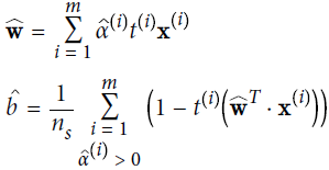
Eliminating w and b from L(w, b, a) using these conditions then gives the dual representation of the maximum margin problem in which we maximize 
with respect to a subject to the constraints 
Here the kernel function is defined by ![]() , landmark at
, landmark at ![]()
Equation 5-6. Dual form of the linear SVM objective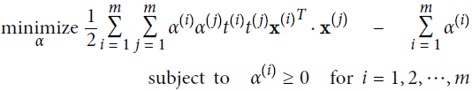
Once you find the vector ![]() that minimizes this equation (using a QP/Quadratic Programming problem solver), you can compute
that minimizes this equation (using a QP/Quadratic Programming problem solver), you can compute ![]() and
and ![]() that minimize the primal problem by using Equation 5-7.
that minimize the primal problem by using Equation 5-7.
Equation 5-7. From the dual solution to the primal solution
##########################################![]()

In order to classify new data points(![]() ) using the trained model, we evaluate the sign of y(x) defined by (7.1). This can be expressed in terms of the parameters {
) using the trained model, we evaluate the sign of y(x) defined by (7.1). This can be expressed in terms of the parameters {![]() } and the kernel function(
} and the kernel function(![]() ) by substituting for w using (7.8) to give
) by substituting for w using (7.8) to give support vector
 ![]() see the following explanations
see the following explanations
a constrained optimization of this form satisfies the Karush-Kuhn-Tucker (KKT) conditions, which in this case require that the following three properties hold 
Thus for every data point, either ![]() = 0 or
= 0 or ![]() = 1. Any data point for which
= 1. Any data point for which ![]() = 0 will not appear in the sum in (7.13) and hence plays no role in making predictions for new data points. The remaining data points are called support vectors, and because they satisfy
= 0 will not appear in the sum in (7.13) and hence plays no role in making predictions for new data points. The remaining data points are called support vectors, and because they satisfy ![]() = 1, they correspond to points that lie on the maximum margin hyperplanes in feature space, as illustrated in Figure 7.1. This property is central to the practical applicability of support vector machines. Once
= 1, they correspond to points that lie on the maximum margin hyperplanes in feature space, as illustrated in Figure 7.1. This property is central to the practical applicability of support vector machines. Once
the model is trained, a significant proportion of the data points can be discarded and only the support vectors retained.
Having solved the quadratic programming problem and found a value for a(=![]() ), we can then determine the value of the threshold parameter b by noting that any support vector
), we can then determine the value of the threshold parameter b by noting that any support vector ![]() satisfies
satisfies ![]() = 1. Using (7.13) this gives
= 1. Using (7.13) this gives![]()
where S denotes the set of indices of the support vectors(![]() ). Although we can solve this equation for b using an arbitrarily chosen support vector
). Although we can solve this equation for b using an arbitrarily chosen support vector ![]() , a numerically more stable solution is obtained by first multiplying through by
, a numerically more stable solution is obtained by first multiplying through by ![]() , making use of
, making use of ![]()
n = 1, and then averaging these equations over all support vectors and solving for b to give
where ![]() is the total number of support vectors.
is the total number of support vectors.
Note: if we not use kernel function(![]() in equation 7.13,
in equation 7.13,![]() , x is one of support vectors
, x is one of support vectors ![]()


![]()
then determine the value of the threshold parameter b by noting that any support vector ![]() satisfies
satisfies ![]() = 1
= 1![]()
![]()
![]()

![]() here N=m
here N=m
![]()
![]()
![]()

![]() where S denotes the set of indices of the support vectors(
where S denotes the set of indices of the support vectors(![]() ), .
), .![]() is the total number of support vectors.
is the total number of support vectors.
##########################################
Once you find the vector ![]() that minimizes this equation (using a QP solver), you can compute
that minimizes this equation (using a QP solver), you can compute ![]() and
and ![]() that minimize the primal problem by using Equation 5-7. (
that minimize the primal problem by using Equation 5-7. (![]() is the total number of support vectors, m denotes the set of indices of the support vectors)
is the total number of support vectors, m denotes the set of indices of the support vectors)
Equation 5-7. From the dual solution to the primal solution
There is still one loose end we must tie. Equation 5-7 shows how to go from the dual solution to the primal solution in the case of a linear SVM classifier, but if you apply the kernel trick you end up with equations that include ![]() . In fact,
. In fact, ![]() must have
must have
the same number of dimensions as ![]() , which may be huge or even infinite, so you can’t compute it. But how can you make predictions without knowing
, which may be huge or even infinite, so you can’t compute it. But how can you make predictions without knowing![]() ? Well, the good news is that you can plug in the formula for
? Well, the good news is that you can plug in the formula for ![]() from Equation 5-7 into the decision function for a new instance
from Equation 5-7 into the decision function for a new instance ![]() , and you get an equation with only dot products between input vectors. This makes it possible to use the kernel trick, once again (Equation 5-11).
, and you get an equation with only dot products between input vectors. This makes it possible to use the kernel trick, once again (Equation 5-11).
Equation 5-11. Making predictions with a kernelized SVM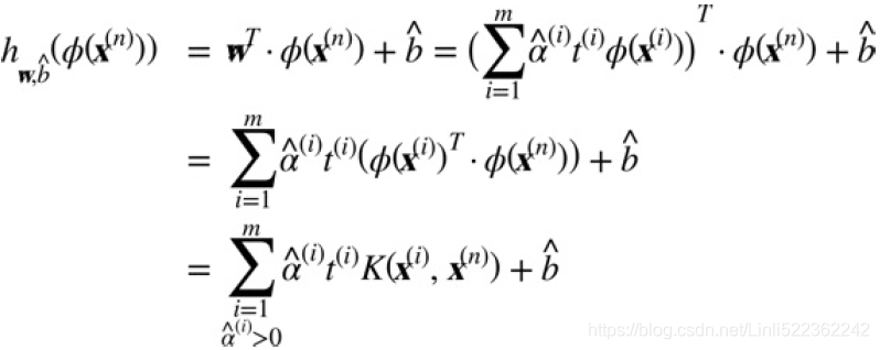
in other words, we use the support vectors as the locations of landmarks in kernel function ![]() .
.
Note that since ![]() ≠ 0 only for support vectors, making predictions involves computing
≠ 0 only for support vectors, making predictions involves computing
the dot product of the new input vector ![]() with only the support vectors
with only the support vectors![]() , not all the training instances. Of course, you also need to compute the bias term b, using the same trick (Equation 5-12).
, not all the training instances. Of course, you also need to compute the bias term b, using the same trick (Equation 5-12).
Equation 5-12. Computing the bias term using the kernel trick
If you are starting to get a headache, it’s perfectly normal: it’s an unfortunate side effects of the kernel trick.
############################################
Quadratic Programming problem
Equation 5-5. Quadratic Programming problem


其中矩阵H对称正定positive definite matrix,A行满秩
首先写出拉格朗日函数:![]()

将上述方程组写成分块矩阵形式:

我们称此方程组的系数矩阵: 为拉格朗日矩阵(Lagrangian function matrix)。
解的表达式为:![]()
如果系数矩阵可逆的话, 则最优解为 x=![]() =
=![]()

至于分块矩阵的求逆公式如下
https://blog.csdn.net/qcyfred/article/details/71598807


#########################
Lagrange Multipliers
Lagrange multipliers, also sometimes called undetermined multipliers, are used to find the stationary points驻点 of a function of several variables subject to(使服从) one or more constraints.

Consider the problem of finding the maximum of a function f(x1, x2) OR ![]() subject to a constraint relating x1 and x2 (or y), which we write in the form
subject to a constraint relating x1 and x2 (or y), which we write in the form ![]() (Sometimes an additive constant is shown separately rather than being included in g, in which case the constraint is written
(Sometimes an additive constant is shown separately rather than being included in g, in which case the constraint is written ![]() , as in Figure 1.(Figure 1: The red curve shows the constraint g(x, y) = c. The blue curves are contours of f(x, y). The point where the red constraint tangentially touches a blue contour is the maximum of f(x, y) along the constraint, since d1 > d2.)
, as in Figure 1.(Figure 1: The red curve shows the constraint g(x, y) = c. The blue curves are contours of f(x, y). The point where the red constraint tangentially touches a blue contour is the maximum of f(x, y) along the constraint, since d1 > d2.)
One approach would be to solve the constraint equation and thus express x2 as a function of x1 in the form x2 = h(x1). This can then be substituted into f(x1, x2) to give a function of x1 alone of the form f(x1, h(x1)). The maximum with respect to x1 could then be found by differentiation in the usual way, to give the stationary value ![]() , with the corresponding value of x2 given by
, with the corresponding value of x2 given by ![]() .
.
One problem with this approach is that it may be difficult to find an analytic solution分析解法 of the constraint equation that allows x2 to be expressed as an explicit function of x1. Also, this approach treats x1 and x2 differently and so spoils损坏 the natural symmetry between these variables.
A more elegant, and often simpler, approach is based on the introduction of a parameter λ called a Lagrange multiplier. We shall motivate促动 this technique from a geometrical perspective. Consider a D-dimensional variable x with components
x1, . . . , xD. The constraint equation g(x) = 0 then represents a (D−1)-dimensional surface in x-space as indicated in Figure E.1.
(Figure E.1 A geometrical picture of the technique of Lagrange multipliers in which we seek to maximize a function f(x), subject to the constraint g(x) = 0. If x is D dimensional, the constraint g(x) = 0 corresponds to a subspace of dimensionality D − 1, indicated by the red curve. The problem can be solved by optimizing the Lagrangian function L(x, λ) = f(x) + λg(x).) Note that if we wish to minimize (rather than maximize) the function f(x) subject to an inequality constraint g(x)
 ![]() 0, then we minimize the Lagrangian function L(x, λ) = f(x) − λg(x) with respect to x, again subject to λ
0, then we minimize the Lagrangian function L(x, λ) = f(x) − λg(x) with respect to x, again subject to λ ![]() 0.
0.
We first note that at any point on the constraint surface the gradient ∇g(x) of the constraint function will be orthogonal to the surface. To see this, consider a point x that lies on the constraint surface, and consider a nearby point x + ![]() that also lies
that also lies
on the surface. If we make a Taylor expansion around x, we have ![]()
Because both x and x+![]() lie on the constraint surface, we have g(x) = g(x+
lie on the constraint surface, we have g(x) = g(x+![]() ) =0 and hence
) =0 and hence ![]() . In the limit
. In the limit ![]() we have
we have ![]() , and because
, and because ![]() is then parallel to the constraint surface g(x) = 0, we see that the vector ∇g is normal正交 to the surface.
is then parallel to the constraint surface g(x) = 0, we see that the vector ∇g is normal正交 to the surface.
Next we seek a point ![]() on the constraint surface such that f(x) is maximized. Such a point must have the property that the vector ∇f(x) is also orthogonal to the constraint surface, as illustrated in Figure E.1, because otherwise we could increase the value of f(x) by moving a short distance along the constraint surface. Thus ∇f and ∇g are parallel (or anti-parallel) vectors, and so there must exist a parameter λ such that
on the constraint surface such that f(x) is maximized. Such a point must have the property that the vector ∇f(x) is also orthogonal to the constraint surface, as illustrated in Figure E.1, because otherwise we could increase the value of f(x) by moving a short distance along the constraint surface. Thus ∇f and ∇g are parallel (or anti-parallel) vectors, and so there must exist a parameter λ such that ![]() where λ
where λ ![]() 0 is known as a Lagrange multiplier. Note that λ can have either sign.
0 is known as a Lagrange multiplier. Note that λ can have either sign.
At this point, it is convenient to introduce the Lagrangian function defined by ![]() The constrained stationarity condition (
The constrained stationarity condition (![]() ) is obtained by setting
) is obtained by setting ![]() . Furthermore, the condition ∂L/∂λ = 0 leads to the constraint equation g(x) = 0.
. Furthermore, the condition ∂L/∂λ = 0 leads to the constraint equation g(x) = 0.
Thus to find the maximum of a function f(x) subject to the constraint g(x) = 0, we define the Lagrangian function given by (E.4 ![]() ) and we then find the stationary point of L(x, λ) with respect to both x and λ. For a D-dimensional vector x, this gives D+1 equations that determine both the stationary point x and the value of λ. If we are only interested in x, then we can eliminate λ from the stationarity equations without needing to find its value (hence the term ‘undetermined multiplier’).
) and we then find the stationary point of L(x, λ) with respect to both x and λ. For a D-dimensional vector x, this gives D+1 equations that determine both the stationary point x and the value of λ. If we are only interested in x, then we can eliminate λ from the stationarity equations without needing to find its value (hence the term ‘undetermined multiplier’).
As a simple example, suppose we wish to find the stationary point of the function ![]() subject to the constraint
subject to the constraint ![]() , as illustrated in Figure E.2. The corresponding Lagrangian function is given by
, as illustrated in Figure E.2. The corresponding Lagrangian function is given by![]()
The conditions for this Lagrangian to be stationary with respect to x1, x2, and λ give the following coupled equations:
Figure E.2 A simple example of the use of Lagrange multipliers in which the aim is to maximize![]()
subject to the constraint g(x1, x2) = 0 where g(x1, x2) = x1 + x2 − 1. The circles show contours of the function f(x1, x2), and the diagonal line shows the constraint surface g(x1, x2) = 0.

Solution of these equations then gives the stationary point as ![]() , and the corresponding value for the Lagrange multiplier is λ = 1.
, and the corresponding value for the Lagrange multiplier is λ = 1.
So far, we have considered the problem of maximizing a function subject to an equality constraint of the form g(x) = 0. We now consider the problem of maximizing f(x) subject to an inequality constraint of the form g(x) ![]() 0, as illustrated in Figure E.3. Illustration of the problem of maximizing f(x) subject to the inequality constraint g(x)
0, as illustrated in Figure E.3. Illustration of the problem of maximizing f(x) subject to the inequality constraint g(x) ![]() 0.
0.
There are now two kinds of solution possible, according to whether the constrained stationary point lies in the region where g(x) > 0, in which case the constraint is inactive, or whether it lies on the boundary g(x) = 0, in which case the constraint is said to be active. In the former case, the function g(x) plays no role and so the stationary condition is simply ∇f(x) = 0. This again corresponds to a stationary point of the Lagrange function (E.4 ![]() ) but this time with λ = 0. The latter case, where the solution lies on the boundary, is analogous to the equality constraint discussed previously and corresponds to a stationary point of the Lagrange function (E.4
) but this time with λ = 0. The latter case, where the solution lies on the boundary, is analogous to the equality constraint discussed previously and corresponds to a stationary point of the Lagrange function (E.4 ![]() ) with
) with ![]() . Now, however, the sign of the Lagrange multiplier is crucial, because the function f(x) will only be at a maximum if its gradient is oriented away from the region g(x) > 0, as illustrated in Figure E.3. We therefore have
. Now, however, the sign of the Lagrange multiplier is crucial, because the function f(x) will only be at a maximum if its gradient is oriented away from the region g(x) > 0, as illustrated in Figure E.3. We therefore have
∇f(x) = −λ∇g(x) for some value of λ > 0.
For either of these two cases, the product λg(x) = 0. Thus the solution to the problem of maximizing f(x) subject to g(x) ![]() 0 is obtained by optimizing the Lagrange function (E.4
0 is obtained by optimizing the Lagrange function (E.4 ![]() ) with respect to x and λ subject to the conditions
) with respect to x and λ subject to the conditions
These are known as the Karush-Kuhn-Tucker (KKT) conditions (Karush, 1939; Kuhn and Tucker, 1951).
Note that if we wish to minimize (rather than maximize) the function f(x) subject to an inequality constraint g(x) ![]() 0, then we minimize the Lagrangian function L(x, λ) = f(x) − λg(x) with respect to x, again subject to λ
0, then we minimize the Lagrangian function L(x, λ) = f(x) − λg(x) with respect to x, again subject to λ ![]() 0.
0.
Finally, it is straightforward to extend the technique of Lagrange multipliers to the case of multiple equality and inequality constraints. Suppose we wish to maximize f(x) subject to ![]() for j = 1, . . . , J, and
for j = 1, . . . , J, and ![]() for k = 1, . . . , K.
for k = 1, . . . , K.
We then introduce Lagrange multipliers {![]() } and {
} and {![]() }, and then optimize the Lagrangian function given by
}, and then optimize the Lagrangian function given by 
subject to ![]()
![]() 0 and
0 and ![]() = 0 for k = 1, . . . , K. Extensions to constrained functional derivatives are similarly straightforward. For a more detailed discussion of the technique of Lagrange multipliers, see Nocedal and Wright (1999).
= 0 for k = 1, . . . , K. Extensions to constrained functional derivatives are similarly straightforward. For a more detailed discussion of the technique of Lagrange multipliers, see Nocedal and Wright (1999).
############################################
#########################
sub-summary;
Linear model: ![]()
1. find the support vectors (![]() =1)as the locations of landmarks in kernel function
=1)as the locations of landmarks in kernel function ![]()
and find the vector α
margin: 几何间隔:即点到面的距离。显然,函数间隔 function margin![]() 与几何间隔Geometric margin
与几何间隔Geometric margin ![]() 只相差||w||倍
只相差||w||倍
Geometric margin: the distance for any data point to the separating hyperplane is![]() >=1 (constraints)
>=1 (constraints)
hard margin:
, constraint: 
we introduce Lagrange multipliers拉格朗日乘数![]() 0, with one multiplier
0, with one multiplier ![]() for each of the constraints in (7.5), giving the Lagrangian function
for each of the constraints in (7.5), giving the Lagrangian function
maximize
https://blog.csdn.net/Linli522362242/article/details/104151351
Eliminating w and b from L(w, b, a) using these conditions then gives the dual representation of the maximum margin problem in which we maximize
with respect to a subject to the constraints
Here the kernel function is defined by ![]() , landmark at
, landmark at ![]()
Equation 5-6. Dual form of the linear SVM objective(==equation 7.10)
The remaining data points are called support vectors, and because they satisfy ![]() = 1 and
= 1 and ![]() >0, they correspond to points that lie on the maximum margin hyperplanes in feature space,
>0, they correspond to points that lie on the maximum margin hyperplanes in feature space,
Once you find the vector α that minimizes this equation (using a QP solver)
Soft margin:
https://blog.csdn.net/Linli522362242/article/details/104151351
We now wish to minimize (7.21) subject to the constraints (7.20) together with. The corresponding Lagrangian is given by 
where {![]() 0} and {
0} and {![]() 0} are Lagrange multipliers. The corresponding set of KKT conditions are given by
0} are Lagrange multipliers. The corresponding set of KKT conditions are given by
where n = 1,...,N.
We now optimize out w, b, and {ξn} making use of the definition (7.1 ![]() ) of y(x) to give
) of y(x) to give
which is identical to the separable case(7.10), except that the constraints are somewhat different. To see what these constraints are, we note that is required because these are Lagrange multipliers. Furthermore, (7.31) together with ![]() implies
implies ![]() We therefore have to minimize (7.32) with respect to the dual variables {
We therefore have to minimize (7.32) with respect to the dual variables { } subject to
for n = 1,...,N, where (7.33) are known as box constraints. This again represents a quadratic programming problem. If we substitute (7.29) into (7.1 ![]() ), we see that predictions for new data points(
), we see that predictions for new data points(![]() ) are again made by using (7.13
) are again made by using (7.13  ).The remaining data points constitute the support vectors
![]() .
.
since these have and hence from (7.25: ![]() ) must satisfy
) must satisfy ![]()
If  < C, then (7.31
 ![]() ) implies that
) implies that  > 0, which from (7.28
 ![]() ) requires ξn = 0 and hence such points(support vectors
) requires ξn = 0 and hence such points(support vectors![]() .) lie on the margin.
.) lie on the margin.
Points with ![]() = C can lie inside the margin and can either be correctly classified
= C can lie inside the margin and can either be correctly classified ![]() if or misclassified if
if or misclassified if ![]() .
.
2. select a kernel function
example1:
Suppose you want to apply a 2nd-degree polynomial transformation to a two dimensional(x1, x2) training set

Notice that the transformed vector is three-dimensional(![]() ,
, ![]() ,
,![]() ) instead of two-dimensional
) instead of two-dimensional![]() .
.
3. Equation 5-12. Computing the bias term using the kernel trick
(![]() is the total number of support vectors, m denotes the set of indices of the support vectors,
is the total number of support vectors, m denotes the set of indices of the support vectors, ![]() ≠ 0)
≠ 0)
4. Making predictions with a kernelized SVM for a new instance ![]()
#########################
Online SVMs
Before concluding this chapter, let’s take a quick look at online SVM classifiers (recall that online learning means learning incrementally, typically as new instances arrive).
For linear SVM classifiers, one method is to use Gradient Descent (e.g., using SGDClassifier) to minimize the cost function in Equation 5-13, which is derived from the primal problem. Unfortunately it converges much more slowly than the methods based on QP.
Equation 5-13. Linear SVM classifier cost function ![]()
The first sum in the cost function will push the model to have a small weight vector w, leading to a larger margin. The second sum![]() computes the total of all margin violations. An instance’s margin violation is equal to 0 if it is located off the street and on the correct side, or else it is proportional成比例的 to the distance to the correct side of the street. Minimizing this term ensures that the model makes the margin violations as small and as few as possible.
computes the total of all margin violations. An instance’s margin violation is equal to 0 if it is located off the street and on the correct side, or else it is proportional成比例的 to the distance to the correct side of the street. Minimizing this term ensures that the model makes the margin violations as small and as few as possible.
######################################
Hinge Loss
t=![]()
The function max(0, 1 – t) is called the hinge loss function (represented below). It is equal to 0 when t ≥ 1; it is equal to 1-t if t<1. Its derivative (slope) is equal to –1 if t < 1 and Its derivative (slope) is equal to 0 if t > 1. It is not differentiable不可微的 at t = 1, but just like for Lasso套索 Regression (see “Lasso Regression”  ) you can still use Gradient Descent
  using any subderivative at t = 0 (i.e., any value between –1 and 0).

y is the labe/class -1/+1
https://www.cnblogs.com/veagau/articles/11876915.html
######################################
It is also possible to implement online kernelized SVMs—for example, using “Incremental and Decremental SVM Learning” or “Fast Kernel Classifiers with Online and Active Learning.” However, these are implemented in Matlab and C++. For largescale
nonlinear problems, you may want to consider using neural networks instead.
1. What is the fundamental idea behind Support Vector Machines?
The fundamental idea behind Support Vector Machines is to fit the widest possible “street” between the classes. In other words, the goal is to have the largest possible margin between the decision boundary that separates the two classes and the training instances. When performing soft margin classification, the SVM searches for a compromise妥协 between perfectly separating the two classes and having the widest possible street (i.e., a few instances may end up on the street). Another key idea is to use kernels when training on nonlinear datasets.
2. What is a support vector?
After training an SVM, a support vector is any instance located on the “street” (see the previous answer), including its border. The decision boundary is entirely determined by the support vectors. Any instance that is not a support vector (i.e., off the street) has no influence whatsoever; you could remove them, add more instances, or move them around, and as long as they stay off the street they won’t affect the decision boundary. Computing the predictions only involves the support vectors, not the whole training set.
3. Why is it important to scale the inputs when using SVMs?
SVMs try to fit the largest possible “street” between the classes (see the first answer), so if the training set is not scaled, the SVM will tend to neglect small features.
https://blog.csdn.net/Linli522362242/article/details/104151351
4. Can an SVM classifier output a confidence score when it classifies an instance? What about a probability?
An SVM classifier can output the distance between the test instance and the decision boundary, and you can use this as a confidence score. However, this score cannot be directly converted into an estimation of the class probability. If you set probability=True when creating an SVM in Scikit-Learn, then after training it will calibrate the probabilities using Logistic Regression on the SVM’s scores (trained by an additional five-fold cross-validation on the training data). This will add the predict_proba() and predict_log_proba() methods to the SVM.
5. Should you use the primal or the dual form of the SVM problem to train a model on a training set with millions of instances and hundreds of features?
the primal form![]() s.t.
s.t. ![]()
Equation 5-6. Dual form of the linear SVM objective (maximize margin classifier)
This question applies only to linear SVMs since kernelized can only use the dual form. The computational complexity of the primal form of the SVM problem is proportional to the number of training instances m, while the computational complexity of the dual form is proportional to a number between ![]() and
and ![]() . So if there are millions of instances, you should definitely use the primal form, because the dual form will be much too slow.
. So if there are millions of instances, you should definitely use the primal form, because the dual form will be much too slow.
6. Say you trained an SVM classifier with an RBF kernel. It seems to underfit the training set: should you increase or decrease γ (gamma)? What about C?
If an SVM classifier trained with an RBF kernel underfits the training set, there might be too much regularization. To decrease it, you need to increase gamma or C (or both).
from sklearn.svm import SVC

gamma1, gamma2 = 0.1, 5
C1, C2 = 0.001,1000
hyperparams = (gamma1, C1), (gamma1, C2), (gamma2, C1), (gamma2,C2)

svm_clfs = []
for gamma, C in hyperparams:
    rbf_kernel_svm_clf = Pipeline([
        ("scaler", StandardScaler()),
        ("svm_clf", SVC(kernel="rbf", gamma=gamma, C=C))
    ])
    rbf_kernel_svm_clf.fit(X,y)
    svm_clfs.append(rbf_kernel_svm_clf)

def plot_predictions(clf, axes):
    x0s = np.linspace(axes[0], axes[1], 100)
    x1s = np.linspace(axes[2], axes[3], 100)
    x0, x1 = np.meshgrid(x0s, x1s)
    X = np.c_[x0.ravel(), x1.ravel()]
    y_pred = clf.predict(X).reshape(x0.shape)
    y_decision = clf.decision_function(X).reshape(x0.shape) #decision broundary
    plt.contourf(x0,x1, y_pred, cmap=plt.cm.brg, alpha=0.2)
    plt.contourf(x0,x1,y_decision,cmap=plt.cm.brg, alpha=0.1)

def plot_dataset(X,y, axes):
    plt.plot(X[:,0][y==0], X[:,1][y==0], "bs")
    plt.plot(X[:,0][y==1], X[:,1][y==1], "g^")
    plt.axis(axes)
    plt.grid(True, which="both")
    plt.xlabel(r"$x_1$", fontsize=20)
    plt.ylabel(r"$x_2$", fontsize=20, rotation=0)

fig, axes = plt.subplots(nrows=2, ncols=2, figsize=(10.5,7))

for i,svm_clf in enumerate(svm_clfs):
    plt.sca( axes[i//2, i%2] )###
    plot_predictions(svm_clf, [-1.5,2.5, -1,1.5])
    plot_dataset(X,y, [-1.5,2.5, -1,1.5])
    gamma, C=hyperparams[i]
    plt.title( r"$\gamma = {},C={}$".format(gamma, C), fontsize=16 )

plt.subplots_adjust(hspace=0.4)
plt.show()

These plots show models trained with different values of hyperparameters gamma (γ) and C. Increasing gamma(γ) makes the bell-shape curve narrower (see the right plot of Figure 5-9), and as a result each instance’s range of influence is smaller: the decision boundary ends up being more irregular, wiggling扭动 around individual instances. Conversely, a small gamma(γ) value makes the bell-shaped curve wider, so instances have a larger range of influence, and the decision boundary ends up smoother. So γ acts like a regularization hyperparameter: if your model is overfitting, you should reduce it, and if it is underfitting, you should increase it (similar to the C hyperparameter).
##############################################
Intuitively, the gamma parameter defines how far the influence of a single training example reaches, with low values meaning ‘far’ and high values meaning ‘close’. The gamma parameters can be seen as the inverse of the radius of influence of samples selected by the model as support vectors. 
The behavior of the model is very sensitive to the gamma parameter. If gamma is too large, the radius of the area of influence of the support vectors only includes the support vector itself and no amount of regularization with C will be able to prevent overfitting.
When gamma is very small, the model is too constrained and cannot capture the complexity or “shape” of the data. The region of influence of any selected support vector would include the whole training set. The resulting model will behave similarly to a linear model with a set of hyperplanes that separate the centers of high density of any pair of two classes.
The C parameter trades off correct classification of training examples against maximization of the decision function’s margin. For larger values of C, a smaller margin will be accepted if the decision function is better at classifying all training points correctly. A lower C will encourage a larger margin, therefore a simpler decision function, at the cost of training accuracy. In other words``C`` behaves as a regularization parameter in the SVM. https://scikit-learn.org/stable/auto_examples/svm/plot_rbf_parameters.html
The first plot is a visualization of the decision function for a variety of parameter values on a simplified classification problem involving only 2 input features and 2 possible target classes (binary classification). Note that this kind of plot is not possible to do for problems with more features or target classes.
The second plot is a heatmap of the classifier’s cross-validation accuracy as a function of C and gamma. For this example we explore a relatively large grid for illustration purposes. In practice, a logarithmic grid from ![]() to
to ![]() is usually sufficient. If the best parameters lie on the boundaries of the grid, it can be extended in that direction in a subsequent search.
is usually sufficient. If the best parameters lie on the boundaries of the grid, it can be extended in that direction in a subsequent search.
For intermediate values, we can see on the second plot that good models can be found on a diagonal of C and gamma. Smooth models (lower gamma values) can be made more complex by increasing the importance of classifying each point correctly (larger C values) hence the diagonal of good performing models.
##############################################
solve the hard margin linear SVM classifier problem using an off-the-shelf QP solver: https://blog.csdn.net/Linli522362242/article/details/104280075
7. How should you set the QP parameters (H, f, A, and b) to solve the soft margin linear SVM classifier problem using an off-the-shelf QP solver?另一种表述如何设置这些参数,把软间隔线性SVM模型转化为二次规划问题

Let’s call the QP parameters for the hard-margin problem H′, f′, A′ and b′ (see “Quadratic Programming”). The QP parameters for the soft-margin problem have m additional parameters (![]() =n + 1 + m ; where n is the number of features ;the +1 is for the bias term; m is the number of training instances.) and m additional constraints (
=n + 1 + m ; where n is the number of features ;the +1 is for the bias term; m is the number of training instances.) and m additional constraints (![]() = 2m). They can be defined like so:
= 2m). They can be defined like so:
- H is equal to H′(the inverse of H matrix), plus m columns of 0s on the right and m rows of 0s at the bottom:

- f is equal to f′ with m additional elements, all equal to the value of the hyperparameter C.
- b is equal to b′ with m additional elements, all equal to 0.
- A is equal to A′, with an extra m × m identity matrix

 appended to the right, just below it, and the rest filled with zeros:

![]() ==>
==>![]() ==>
==>
![]() ==>
==>![]() ==>
==> note
note![]() is an m dimensions of row vector with the ith element and value is 1, the other elements are 0s;
is an m dimensions of row vector with the ith element and value is 1, the other elements are 0s; ![]() ==>
==>![]()
![]() 0==>(0,0,
0==>(0,0,![]() )
)![]()
![]() 0
0
Then conbines two constraints: 

8. Train a LinearSVC on a linearly separable dataset. Then train an SVC and a SGDClassifier on the same dataset. See if you can get them to produce roughly the same model.
Let's use the Iris dataset: the Iris Setosa and Iris Versicolor classes are linearly separable.
Equation 5-13. Linear SVM classifier cost function ![]()
rom sklearn import datasets

iris = datasets.load_iris()
X = iris['data'][:,(2,3)] #petal length, petal width
y = iris['target']

setosa_or_versicolor = (y==0) | (y==1)
X = X[setosa_or_versicolor]
y = y[setosa_or_versicolor]
from sklearn.svm import SVC, LinearSVC
from sklearn.linear_model import SGDClassifier
from sklearn.preprocessing import StandardScaler
C=5
alpha = 1/( C*len(X) )
lin_clf = LinearSVC(loss="hinge", C=C, random_state=42)#‘hinge’ is the standard SVM loss
svm_clf = SVC(kernel="linear", C=C)
sgd_clf = SGDClassifier(loss="hinge", learning_rate="constant", eta0=0.001, alpha=alpha,
max_iter=1000, tol=1e-3, random_state=42)
scaler = StandardScaler()
X_scaled = scaler.fit_transform(X)
lin_clf.fit(X_scaled, y)
svm_clf.fit(X_scaled, y)
sgd_clf.fit(X_scaled, y)
print("LinearSVC: ", lin_clf.intercept_, lin_clf.coef_)
print("SVC: ", svm_clf.intercept_, svm_clf.coef_)
print("SGDClassifier(alpha={:.5f}):".format(sgd_clf.alpha), sgd_clf.intercept_, sgd_clf.coef_)
Let's plot the decision boundaries of these three models:
At first, we have to understand that plotting the data points use original data points
Secondly, the Separating hyperplane w0*x0 + w1*x1 + b =0 ==> x1 = (-w0/w1)*x0 + (-b/w1) = new_w1*x0 + new_b
finally, we plot the decision boundary line which is from two scaled vectors(two data points), so we have to do scaler.inverse_transform() with known X_length and X_width= new_w1*X_length + new_b
# Compute the slope and bias of each decision boundary
# Separating hyperplane w0*x0 + w1*x1 + b =0 ==> x1 = (-w0/w1)*x0 + (-b/w1) = w1*x0 + b1    ########
# LinearSVC:                    [0.28474027] [[1.0536456  1.09903032]]
w1 = -lin_clf.coef_[0,0] / lin_clf.coef_[0,1]
b1 = -lin_clf.intercept_[0] / lin_clf.coef_[0,1]
# SVC:                          [0.31896852] [[1.1203284  1.02625193]]
w2 = -svm_clf.coef_[0,0] / svm_clf.coef_[0,1]
b2 = -svm_clf.intercept_[0] / svm_clf.coef_[0,1]
# SGDClassifier(alpha=0.00200): [0.117] [[0.77714169 0.72981762]]
w3 = -sgd_clf.coef_[0,0] / sgd_clf.coef_[0,1]
b3 = -sgd_clf.intercept_[0] / sgd_clf.coef_[0,1]

# Transform the decision boudary lines back to the original scale
line1 = scaler.inverse_transform([ [-10, -10*w1 + b1], [10, 10*w1 + b1] ])#([ [x0, w1*x0 +b1],[x0, w1*x0 +b1] ])
line2 = scaler.inverse_transform([ [-10, -10*w2 + b2], [10, 10*w2 + b2] ])
line3 = scaler.inverse_transform([ [-10, -10*w3 + b3], [10, 10*w3 + b3] ])

# Plot all three decision boundaries
plt.figure( figsize=(11,4) )
plt.plot( line1[:,0], line1[:,1], "k:", label="LinearSVC" )
plt.plot( line2[:,0], line2[:,1], "b--", label="SVC", linewidth=2 )
plt.plot( line3[:,0], line3[:,1], "r-", label="SGDClassifier" )

plt.plot(X[:,0][y==1], X[:,1][y==1], "bs") # label="Iris versicolor"
plt.plot(X[:,0][y==0], X[:,1][y==0], "yo") # label="Iris setosa"

plt.xlabel("Petal length", fontsize=14)
plt.ylabel("Petal width", fontsize=14)
plt.legend(loc="upper center", fontsize=14)
plt.axis([0,5.5, 0,2])

plt.show()
9. Exercise: train an SVM classifier on the MNIST dataset. Since SVM classifiers are binary classifiers, you will need to use one-versus-all to classify all 10 digits. You may want to tune the hyperparameters using small validation sets to speed up the process. What accuracy can you reach?
First, let's load the dataset and split it into a training set and a test set. We could use train_test_split() but people usually just take the first 60,000 instances for the training set, and the last 10,000 instances for the test set (this makes it possible to compare your model's performance with others):
from sklearn.datasets import fetch_openml
#https://blog.csdn.net/Linli522362242/article/details/103786116
mnist = fetch_openml('mnist_784', version=1, cache=True)

X, y = mnist["data"], mnist["target"].astype(np.uint8)

X_train, X_test, y_train, y_test = X[:60000], X[60000:], y[:60000], y[60000:]
Let’s also shuffle the training set; this will guarantee that all cross-validation folds will be similar (you don’t want one fold to be missing some digits). Moreover, some learning algorithms are sensitive to the order of the training instances, and they perform poorly if they get many similar instances in a row.
shuffle_index = np.random.permutation( len(X_train) )
X_train, y_train = X_train[shuffle_index], y_train[shuffle_index]
Let's start simple, with a linear SVM classifier. It will automatically use the One-vs-All (also called One-vs-the-Rest, OvR) strategy, so there's nothing special we need to do. Easy!
Warning: this may take a few minutes depending on your hardware.
lin_clf = LinearSVC(random_state=42)
lin_clf.fit(X_train, y_train)
Let's make predictions on the training set and measure the accuracy (we don't want to measure it on the test set yet, since we have not selected and trained the final model yet):
from sklearn.metrics import accuracy_score

y_pred = lin_clf.predict(X_train)
accuracy_score(y_train, y_pred)![]()
Okay, 89.5% accuracy on MNIST is pretty bad. This linear model is certainly too simple for MNIST, but perhaps we just needed to scale the data first:
scaler = StandardScaler()
X_train_scaled = scaler.fit_transform( X_train.astype(np.float32) )
X_test_scaled = scaler.transform( X_test.astype(np.float32) )
then train a simple LinearSVR :
lin_clf = LinearSVC( random_state=42 )
lin_clf.fit(X_train_scaled, y_train)
y_pred = lin_clf.predict(X_train_scaled)
accuracy_score(y_train, y_pred)![]() #accuracy_score
#accuracy_score
That's much better(we cut the error rate by about 25%), but still not great at all for MNIST. If we want to use an SVM, we will have to use a kernel. Let's try an SVC with an RBF kernel (the default).
Note: to be future-proof we set gamma="scale" since it will be the default value in Scikit-Learn 0.22.
svm_clf = SVC(gamma="scale", kernel="rbf")
svm_clf.fit( X_train_scaled[:10000], y_train[:10000] )
y_pred = svm_clf.predict( X_train_scaled )
accuracy_score(y_train, y_pred)![]()
That's promising, we get better performance even though we trained the model on 6 times less data. Let's tune the hyperparameters by doing a randomized search with cross validation. We will do this on a small dataset just to speed up the process:
#######################
In probability and statistics, the reciprocal distribution, also known as the log-uniform distribution, is a continuous probability distribution. It is characterised by its probability density function, within the support of the distribution, being proportional to the reciprocal of the variable.
https://en.wikipedia.org/wiki/Reciprocal_distribution
#######################
from sklearn.model_selection import RandomizedSearchCV
from scipy.stats import reciprocal, uniform

param_distributions = { "gamma": reciprocal(0.001,0.1), "C":uniform(1,10) }
rnd_search_cv = RandomizedSearchCV( svm_clf, param_distributions, n_iter=10, verbose=2, cv=3 )
rnd_search_cv.fit( X_train_scaled[:1000], y_train[:1000] )
... ...
rnd_search_cv.best_estimator_
rnd_search_cv.best_score_![]()
rnd_search_cv.best_estimator_.fit(X_train_scaled, y_train)
y_pred = rnd_search_cv.best_estimator_.predict(X_train_scaled)
accuracy_score(y_train, y_pred)![]()
Ah, this looks good! Let's select this model. Now we can test it on the test set:
y_pred = rnd_search_cv.best_estimator_.predict(X_test_scaled)
accuracy_score(y_test, y_pred)![]()
Not too bad, but apparently the model is overfitting slightly(In test set, the accuracy_score is 0.972 which is lower than the accuracy_score(0.9995) in training set). It's tempting to tweak the hyperparameters a bit more (e.g. decreasing C and/or gamma), but we would run the risk of overfitting the test set. Other people have found that the hyperparameters C=5 and gamma=0.005 yield even better performance (over 98% accuracy). By running the randomized search for longer and on a larger part of the training set, you may be able to find this as well.
10. Exercise: train an SVM regressor on the California housing dataset.
Let's load the dataset using Scikit-Learn's fetch_california_housing() function:
from sklearn.datasets import fetch_california_housing

housing = fetch_california_housing()
X = housing["data"]
y = housing["target"]![]()
Split it into a training set and a test set:
from sklearn.model_selection import train_test_split

X_train, X_test, y_train, y_test = train_test_split(X, y, test_size=0.2, random_state=42)
to scale the data:
from sklearn.preprocessing import StandardScaler

scaler = StandardScaler()
X_train_scaled = scaler.fit_transform(X_train)
X_test_scaled = scaler.transform(X_test)
Let's train a simple LinearSVR first:
from sklearn.svm import LinearSVR

lin_svr = LinearSVR(random_state=42)
lin_svr.fit(X_train_scaled, y_train)
Let's see how it performs on the training set:
from sklearn.metrics import mean_squared_error

y_pred = lin_svr.predict(X_train_scaled)
mse = mean_squared_error(y_train, y_pred)
mse![]()
Let's look at the RMSE:
np.sqrt(mse)![]()
In this training set, the targets are tens of thousands of dollars. The RMSE gives a rough idea of the kind of error you should expect (with a higher weight for large errors): so with this model we can expect errors somewhere around $10,000(0.98*10,000). Not great. Let's see if we can do better with an RBF Kernel. We will use randomized search with cross validation to find the appropriate hyperparameter values for C and gamma:
from sklearn.svm import SVR
from sklearn.model_selection import RandomizedSearchCV
from scipy.stats import reciprocal, uniform

param_distributions = { "gamma": reciprocal(0.001, 0.1), "C":uniform(1,10) }
rnd_search_cv = RandomizedSearchCV( SVR(), param_distributions, n_iter=10, verbose=2, cv=3, random_state=42 )
rnd_search_cv.fit(X_train_scaled, y_train)
... ...
rnd_search_cv.best_estimator_
Now let's measure the RMSE on the training set:
y_pred = rnd_search_cv.best_estimator_.predict(X_train_scaled)
mse = mean_squared_error(y_train,y_pred)
np.sqrt(mse)![]()
Looks much better than the linear model(the expect error is 0.57 *10,000 < 0.977*10,000). Let's select this model and evaluate it on the test set:
y_pred = rnd_search_cv.best_estimator_.predict(X_test_scaled)
mse = mean_squared_error(y_test, y_pred)
np.sqrt(mse)![]()
