A Support Vector Machine (SVM) is a very powerful and versatile多种功能的 Machine Learning model, capable of performing linear or nonlinear classification, regression, and even outlier detection. It is one of the most popular models in Machine Learning, and anyone interested in Machine Learning should have it in their toolbox. SVMs are particularly well suited for classification of complex but small- or medium-sized datasets.
#############################################################
Distance from point Q=(x1,y1,z1) to plane Ax+By+Cz+D=0
the distance d of a point Q=(x1,y1,z1) to a plane is determined by normal vector(法向量) ![]() OR N=(A,B,C) and point P=(x0,y0,z0). The equation for the plane determined by N and P is A(x−x0)+B(y−y0)+C(z−z0)=0, which we could write as Ax+By+Cz+D=0, where D=−Ax0−By0−Cz=0. (Ax+By+Cz −A*x0−B*y0−C*z0=0)
OR N=(A,B,C) and point P=(x0,y0,z0). The equation for the plane determined by N and P is A(x−x0)+B(y−y0)+C(z−z0)=0, which we could write as Ax+By+Cz+D=0, where D=−Ax0−By0−Cz=0. (Ax+By+Cz −A*x0−B*y0−C*z0=0)
a unit normal vector N: ![]()
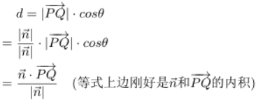
the distance d >=0 from Q to the plane, is simply the length of the projection of vector PQ onto the unit normal vector N.
note: the dot product(内积)![]() and
and ![]() =
= ![]()
 ==>
==> 
the plane  Ax+By+Cz+D=0 is a separating hyperplane(N=(A,B,C) is vector W, b==D ) in Support Vector Machines, and it has another form
 ![]() =0 OR
=0 OR ![]() =0
=0
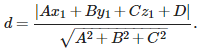
the formula of the distance for any data point to the separating hyperplane is ![]() >=1 (constraints)note A = X (X is a vector, a data point with some features, x0, x1 ... Xn, the following example just use two features)
>=1 (constraints)note A = X (X is a vector, a data point with some features, x0, x1 ... Xn, the following example just use two features)
All this w and b stuff describes the separating line, or hyperplane, for our data.
#############################################################
Linear SVM Classification
The fundamental idea behind SVMs is best explained with some pictures. Figure 5-1 shows part of the iris dataset that was introduced at the end of https://blog.csdn.net/Linli522362242/article/details/104097191. The two classes can clearly be separated easily with a straight line (they are linearly separable). The left plot shows the decision boundaries of three possible linear classifiers. The model whose decision boundary is represented by the dashed line is so bad that it does not even separate the classes properly. The other two models work perfectly on this training set, but their decision boundaries come so close to the instances that these models will probably not perform as well on new instances. In contrast, the solid line in the plot on the right represents the decision boundary of an SVM classifier; this line not only separates the two classes but also stays as far
away from the closest training instances as possible. You can think of an SVM classifier as fitting the widest possible street (represented by the parallel dashed lines) between the classes. This is called large margin classification最大间隔分类.
from sklearn.svm import SVC
from sklearn import datasets

iris = datasets.load_iris()
X = iris["data"][:, (2,3)] # petal length, petal width
y = iris["target"]

setosa_or_versicolor = (y==0) | (y==1)
X = X[setosa_or_versicolor]
y = y[setosa_or_versicolor]

#SVM Classifier model #without using StandardScaler() to process the dataset
svm_clf = SVC(kernel="linear", C=float("inf"))
svm_clf.fit(X,y)
svm_clf.support_vectors_ #the instances(or the points) located on the edge of the street(called large margin)![]()
########################################################extra matrials
#separating hyperplane w0*x0 + w1*x1 + b=0: ==> x1 == -w0/w1*x0 -b/w1 ; In other words, we use the value range of feature x0 to find the value range of feature x1 for plotting the separating hyperplane.
#Note: Here: I use the support vectors to plot the support hyperplanes
gutter_up = -w[0]/w[1] *x0 + (svm_clf.support_vectors_[1][1] -(-w[0]/w[1]*svm_clf.support_vectors_[1][0]))
gutter_down = -w[0]/w[1] *x0 + (svm_clf.support_vectors_[0][1] -(-w[0]/w[1]*svm_clf.support_vectors_[0][0]))
# Bad models
x0 = np.linspace(0, 5.5, 200)
pred_1 = 5*x0 - 20
pred_2 = x0 - 1.8
pred_3 = 0.1 * x0 + 0.5

def plot_svc_decision_boundary(svm_clf, xmin, xmax):
    w = svm_clf.coef_[0] #array([1.29411744, 0.82352928])
    b = svm_clf.intercept_[0] #-3.78823471

    # At the decision boundary, w0*x0 + w1*x1 + b = 0 ==> x1 == -w0/w1*x0 -b/w1
    x0 = np.linspace(xmin, xmax, 200)
    decision_boundary = -w[0]/w[1] *x0 - b/w[1] #x1 #get the separating hyperplane

    #upper-support hyperplane: w0*x0 + w1*x1 + b=1
    #lower-support hyperplane: w0*x0 + w1*x1 + b=-1
    #svm_clf.support_vectors_
    #array([[1.9, 0.4],   #lower-support vector
    #       [3. , 1.1]])  #upper-support vector
    margin = 1/w[1] #vertical move
    #gutter_up = decision_boundary + margin          #-w[0]/w[1]*x0 -b/w[1] +1/w[1]
    gutter_up = -w[0]/w[1] *x0 + (svm_clf.support_vectors_[1][1] -(-w[0]/w[1]*svm_clf.support_vectors_[1][0]))
    #gutter_down = decision_boundary - margin         #-w[0]/w[1]*x0 -b/w[1] -1/w[1]
    gutter_down = -w[0]/w[1] *x0 + (svm_clf.support_vectors_[0][1] -(-w[0]/w[1]*svm_clf.support_vectors_[0][0]))
    svs = svm_clf.support_vectors_ #the instances(or the points) located on the edge of the street(called large margin)
    plt.scatter(svs[:,0], svs[:,1], s=180, facecolor='#FFAAAA')
    plt.plot(x0, decision_boundary, "k-", linewidth=2)
    plt.plot(x0, gutter_up, "b--", linewidth=2)
    plt.plot(x0, gutter_down, "k--", linewidth=2)
                                  #figsize for subplot
fig, axes = plt.subplots(ncols=2, figsize=(10,2.7), sharey=True)

plt.sca(axes[0])
plt.plot(x0, pred_1, "g--", linewidth=2)
plt.plot(x0, pred_2, "m-", linewidth=2)
plt.plot(x0, pred_3, "r-", linewidth=2)
plt.plot(X[:,0][y==1], X[:,1][y==1], "bs", label="Iris versicolor")
plt.plot(X[:,0][y==0], X[:,1][y==0], "yo", label="Iris setosa")
plt.xlabel("Petal length", fontsize=14)
plt.ylabel("Petal width", fontsize=14)
plt.legend(loc="upper left", fontsize=14)
plt.axis([0,5.5, 0,2])

plt.sca(axes[1])
plot_svc_decision_boundary(svm_clf, 0, 5.5)#################call function
plt.plot(X[:,0][y==1], X[:,1][y==1], "bs")
plt.plot(X[:,0][y==0], X[:,1][y==0], "yo")
plt.xlabel("Petal length", fontsize=14)
plt.axis([0,5.5, 0,2])

plt.title("Figure 5-1. Large margin classification")
plt.show()
##########################################################################
#separating hyperplane w0*x0 + w1*x1 + b=0: ==> x1 == -w0/w1*x0 -b/w1 ; In other words, we use the value range of feature x0 to find the value range of feature x1
upper-support hyperplane: w0*x0 + w1*x1 + b=1 ==> gutter_up = -w[0]/w[1]*x0 -b/w[1] +1/w[1]
lower-suppert hyperplane: w0*x0 + w1*x1 + b=-1 ==> gutter_down = -w[0]/w[1]*x0 -b/w[1] -1/w[1]
# Bad models
x0 = np.linspace(0, 5.5, 200)
pred_1 = 5*x0 - 20
pred_2 = x0 - 1.8
pred_3 = 0.1 * x0 + 0.5

def plot_svc_decision_boundary(svm_clf, xmin, xmax):
    w = svm_clf.coef_[0] #array([1.29411744, 0.82352928])
    b = svm_clf.intercept_[0] #-3.78823471

    # At the decision boundary, w0*x0 + w1*x1 + b = 0 ==> x1 == -w0/w1*x0 -b/w1
    x0 = np.linspace(xmin, xmax, 200)
    decision_boundary = -w[0]/w[1] *x0 - b/w[1] #x1 #get the separating hyperplane

    #upper-support hyperplane: w0*x0 + w1*x1 + b=1
    #lower-suppert hyperplane: w0*x0 + w1*x1 + b=-1
    #svm_clf.support_vectors_
    #array([[1.9, 0.4],   #lower-support vector
    #       [3. , 1.1]])  #upper-support vector
    margin = 1/w[1] #vertical move
    gutter_up = decision_boundary + margin          #-w[0]/w[1]*x0 -b/w[1] +1/w[1]
    #gutter_up = -w[0]/w[1] *x0 + (svm_clf.support_vectors_[1][1] -(-w[0]/w[1]*svm_clf.support_vectors_[1][0]))
    gutter_down = decision_boundary - margin         #-w[0]/w[1]*x0 -b/w[1] -1/w[1]
    #gutter_down = -w[0]/w[1] *x0 + (svm_clf.support_vectors_[0][1] -(-w[0]/w[1]*svm_clf.support_vectors_[0][0]))
    svs = svm_clf.support_vectors_ #the instances(or the points) located on the edge of the street(called large margin)
    plt.scatter(svs[:,0], svs[:,1], s=180, facecolor='#FFAAAA')
    plt.plot(x0, decision_boundary, "k-", linewidth=2)
    plt.plot(x0, gutter_up, "b--", linewidth=2)
    plt.plot(x0, gutter_down, "k--", linewidth=2)
                                  #figsize for subplot
fig, axes = plt.subplots(ncols=2, figsize=(10,2.7), sharey=True)

plt.sca(axes[0])
plt.plot(x0, pred_1, "g--", linewidth=2)
plt.plot(x0, pred_2, "m-", linewidth=2)
plt.plot(x0, pred_3, "r-", linewidth=2)
plt.plot(X[:,0][y==1], X[:,1][y==1], "bs", label="Iris versicolor")
plt.plot(X[:,0][y==0], X[:,1][y==0], "yo", label="Iris setosa")
plt.xlabel("Petal length", fontsize=14)
plt.ylabel("Petal width", fontsize=14)
plt.legend(loc="upper left", fontsize=14)
plt.axis([0,5.5, 0,2])

plt.sca(axes[1])
plot_svc_decision_boundary(svm_clf, 0, 5.5)
plt.plot(X[:,0][y==1], X[:,1][y==1], "bs")
plt.plot(X[:,0][y==0], X[:,1][y==0], "yo")
plt.xlabel("Petal length", fontsize=14)
plt.axis([0,5.5, 0,2])

plt.title("Figure 5-1. Large margin classification")
plt.show()
Notice that adding more training instances(![]() or
or  )“off the street” will not affect the decision boundary(the solid line) at all: it is fully determined (or “supported”) by the instances located on the edge of the street. These instances are called the support vectors (they are circled in Figure 5-1).
#######################################
WARNING
SVMs are sensitive to the feature scales缩放, as you can see in Figure 5-2: on the left plot, the vertical scale比例 is much larger than the horizontal scale, so the widest possible street is close to horizontal. After feature scaling特征缩放 (e.g., using Scikit-Learn’s StandardScaler), the decision boundary looks much better (on the right plot).
#######################################
Xs = np.array([ [1,50], [5, 20], [3,80], [5,60] ]).astype(np.float64)
ys = np.array([  0,      0,       1,      1])
svm_clf = SVC(kernel="linear", C=100)
svm_clf.fit(Xs, ys)

plt.figure( figsize=(9,2.7) )

plt.subplot(121)
plt.plot(Xs[:,0][ys==1], Xs[:,1][ys==1], "bo")
plt.plot(Xs[:,0][ys==0], Xs[:,1][ys==0], "ms")
plot_svc_decision_boundary(svm_clf, 0, 6)
plt.xlabel('$x_0$', fontsize=20)
plt.ylabel('$x_1$ ', fontsize=20, rotation=0)
plt.title("Unscaled", fontsize=16)
plt.axis([0,6, 0,90])

from sklearn.preprocessing import StandardScaler
scaler = StandardScaler()
X_scaled = scaler.fit_transform(Xs)
svm_clf.fit(X_scaled, ys)

plt.subplot(122)
plt.plot(X_scaled[:,0][ys==1], X_scaled[:,1][ys==1], "bo")
plt.plot(X_scaled[:,0][ys==0], X_scaled[:,1][ys==0], "ms")
plot_svc_decision_boundary(svm_clf, -2,2)
plt.xlabel("$x_0$", fontsize=20)
plt.ylabel("$x'_1$ ", fontsize=20, rotation=0 )
plt.title("Scaled", fontsize=16)
plt.axis([-2,2, -2,2])
plt.show()
Figure 5-2. Sensitivity to feature scales

Soft Margin Classification
If we strictly impose that all instances be off the street and on the right side, this is called hard margin classification. There are two main issues with hard margin classification. First, it only works if the data is linearly separable, and second it is quite sensitive to outliers. Figure 5-3 shows the iris dataset with just one additional outlier: on the left, it is impossible to find a hard margin, and on the right the decision boundary ends up very different from the one we saw in Figure 5-1 without the outlier, and it will probably not generalize as well.
X_outliers = np.array([ [3.4, 1.3], [3.2, 0.8] ])
y_outliers = np.array([0,0])
Xo1 = np.r_[ X, X_outliers[:1] ]
yo1 = np.r_[ y, y_outliers[:1] ]
Xo2 = np.r_[ X, X_outliers[1:] ]
yo2 = np.r_[ y, y_outliers[1:] ]
                                #for subplot
fig,axes = plt.subplots(ncols=2, figsize=(10, 2.7), sharey=True)

plt.sca(axes[0])
plt.plot( Xo1[:,0][yo1==1], Xo1[:,1][yo1==1], "bs" )
plt.plot( Xo1[:,0][yo1==0], Xo1[:,1][yo1==0], "yo" )
plt.text(0.3, 1.0, "Impossible!", fontsize=24, color="red")
plt.xlabel("Petal length", fontsize=14)
plt.ylabel("Petal width", fontsize=14)
plt.annotate("Outlier",
             xy=(X_outliers[0][0], X_outliers[0][1]),
             xytext=(2.5,1.7),
             ha="center",
             arrowprops=dict(facecolor="black", shrink=0.1),
             fontsize=16,
            )
plt.axis([0, 5.5, 0,2])
plt.title("Figure 5-3. Hard margin sensitivity to outliers")

svm_clf2 = SVC(kernel="linear", C=10**9)
svm_clf2.fit(Xo2, yo2)

plt.sca(axes[1])
plt.plot(Xo2[:,0][yo2==1], Xo2[:,1][yo2==1], "bs")
plt.plot(Xo2[:,0][yo2==0], Xo2[:,1][yo2==0], "yo")
plot_svc_decision_boundary(svm_clf2, 0, 5.5)
plt.xlabel("Petal length", fontsize=14)
plt.annotate("Outlier",
             xy=(X_outliers[1][0], X_outliers[1][1]),
             xytext=(3.2, 0.08),
             ha="center",
             arrowprops=dict(facecolor="black", shrink=0.1),
             fontsize=16,
            )
plt.axis([0,5.5, 0,2])
plt.show()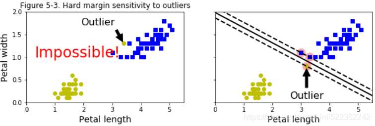
To avoid these issues it is preferable to use a more flexible model. The objective is to find a good balance between keeping the street as large as possible and limiting the margin violations (i.e., instances that end up in the middle of the street or even on the wrong side). This is called soft margin classification.
##########################why the class label is -1 or 1 ##### extra
Why did we switch from class labels of 0 and 1 to -1 and 1? This makes the math manageable, because -1 and 1 are only different by the sign. We can write a single equation![]() (Note:our constraint is
(Note:our constraint is ![]() will be 1.0 or greater)to describe the margin or how close a data point is to our separating hyperplane and not have to worry if the data is in the -1 or +1 class.
will be 1.0 or greater)to describe the margin or how close a data point is to our separating hyperplane and not have to worry if the data is in the -1 or +1 class.
When we’re doing this and deciding where to place the separating line, this margin is calculated by label*(![]() +b). This is where the -1 and 1 class labels help out. If a point is far away from the separating plane on the positive side, then
+b). This is where the -1 and 1 class labels help out. If a point is far away from the separating plane on the positive side, then ![]() +b will be a large positive number, and label*(
+b will be a large positive number, and label*(![]() +b) will give us a large positive number. If it’s far from the negative side and has a negative label (means
+b) will give us a large positive number. If it’s far from the negative side and has a negative label (means ![]() +b will be a negative number), label*(wTx+b) will also give us a large positive number.
+b will be a negative number), label*(wTx+b) will also give us a large positive number.![]()
################################################
########################### Maximum Margin Classifiers
linear models: ![]() OR
OR ![]()
where ![]() denotes a fixed feature-space transformation, and we have made the bias parameter b explicit. Note that we shall shortly introduce a dual representation expressed in terms of kernel functions, which avoids having to work explicitly in feature space. The training data set comprises N input vectors x1,..., xN , with corresponding target values t1,...,tN where tn ∈ {−1, 1}, and new data points x are classified according to the sign of y(x). ######class label
denotes a fixed feature-space transformation, and we have made the bias parameter b explicit. Note that we shall shortly introduce a dual representation expressed in terms of kernel functions, which avoids having to work explicitly in feature space. The training data set comprises N input vectors x1,..., xN , with corresponding target values t1,...,tN where tn ∈ {−1, 1}, and new data points x are classified according to the sign of y(x). ######class label
From the above figure, we know the fact that the all support vectors are not always our data points(see right figure), but at least one of data points is the support vector.
The goal now is to find the w and b values that will define our classifier. To do this, we must find the points with the smallest margin  . These are the support vectors. Then, when we find the points with the smallest margin, we must maximize that margin
 ![]() .
. OR
OR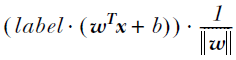
The margin is given by the perpendicular distance to the closest point ![]() from the data set, and we wish to optimize the parameters w and b in order to maximize this distance. Thus the maximum margin solution is found by solving
from the data set, and we wish to optimize the parameters w and b in order to maximize this distance. Thus the maximum margin solution is found by solving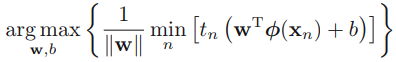
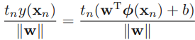
where we have taken the factor 1/w outside the optimization over n because w does not depend on n. Direct solution of this optimization problem would be very complex, and so we shall convert it into an equivalent problem that is much easier to solve. To do this we note that if we make the rescaling w → κw and b → κb, then the distance from any point xn to the decision surface, given by ![]() y(xn)/|w|, is unchanged. We can use this freedom to set
y(xn)/|w|, is unchanged. We can use this freedom to set
![]() ###support hyperplanes###
###support hyperplanes### ![]() =1 =|y|
=1 =|y|
for the point that is closest to the surface. In this case, all data points will satisfy the constraints ![]() OR
OR ![]() -1 >=0
-1 >=0
This is known as the canonical representation of the decision hyperplane(separating hyperplane). In the case of data points for which the equality holds, the constraints are said to be active ![]() , whereas for the remainder they are said to be inactive. By definition, there will always be at least one active constraint(means at least one of data points is the support vector), because there will always be a closest point, and once the margin has been maximized
, whereas for the remainder they are said to be inactive. By definition, there will always be at least one active constraint(means at least one of data points is the support vector), because there will always be a closest point, and once the margin has been maximized ![]() there will be at least two active constraints(lead to y=-1 and y=1 ). The optimization problem then simply requires that we maximize
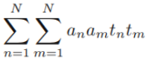
there will be at least two active constraints(lead to y=-1 and y=1 ). The optimization problem then simply requires that we maximize ![]() (inactive constraint), which is equivalent to minimizing
(inactive constraint), which is equivalent to minimizing ![]() , and so we have to solve the optimization problem
, and so we have to solve the optimization problem  The factor of
 ![]() is included for later convenience. This is an example of a quadratic programming problem in which we are trying to minimize a quadratic function subject to a set of linear inequality constraints. It appears that the bias parameter b has disappeared from the optimization. However, it is determined implicitly via the constraints, because these require that changes to|w|be compensated by changes to b. We shall see how this works shortly.
is included for later convenience. This is an example of a quadratic programming problem in which we are trying to minimize a quadratic function subject to a set of linear inequality constraints. It appears that the bias parameter b has disappeared from the optimization. However, it is determined implicitly via the constraints, because these require that changes to|w|be compensated by changes to b. We shall see how this works shortly.
######################################
sub-Summary: to solve
-->At first, ![]() since the constraints
since the constraints ![]() , so the minimum value is 1 which is lead by the support vectors(find them at first)
, so the minimum value is 1 which is lead by the support vectors(find them at first)
Then maximize ![]() ==> maximize
==> maximize ![]() ==> is equivalent to minimizing
==> is equivalent to minimizing ![]() ==>
==> ![]()
######################################Lagrange multiplier拉格朗日乘数
In order to solve this constrained optimization (maximize) problem, we introduce Lagrange multipliers拉格朗日乘数![]() 0, with one multiplier
0, with one multiplier ![]() for each of the constraints in (7.5), giving the Lagrangian function
for each of the constraints in (7.5), giving the Lagrangian function 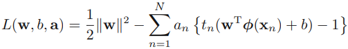 ###we put the constraints together
where a = ![]() . Note the minus sign in front of the Lagrange multiplier term, because we are minimizing with respect to w and b, and maximizing with respect to
. Note the minus sign in front of the Lagrange multiplier term, because we are minimizing with respect to w and b, and maximizing with respect to ![]() . Setting the derivatives of L(w, b, a) with respect to w and b equal to zero, we obtain the following two conditions
. Setting the derivatives of L(w, b, a) with respect to w and b equal to zero, we obtain the following two conditions
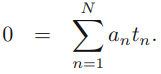
the partial derivatives of L (w, b, a)=0 ==>![]() ==>
==>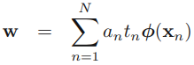
the partial derivatives of L (w, b, a)=0 ==>![]() ==>
==> 
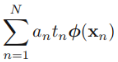
Eliminating w and b from L(w, b, a) using these conditions
replaced with ![]()
![]() ==
==![]()
![]() * w ==
* w ==![]()
 *
* ![]()
![]()
![]()
![]()
![]()
and, 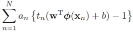 ==
==

 +
+ 
![]() +
+ 
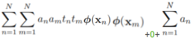
==>  +0+
+0+
Then,
![]()
 --
--  ==>
==>
 ==>
==> 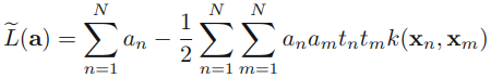
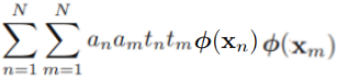
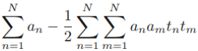
then gives the dual representation of the maximum margin problem in which we maximize ![]()
with respect to a subject to the constraints 
Here the kernel function is defined by ![]() or
or ![]() Again, this takes the form of a quadratic programming problem in which we optimize(maximize) a quadratic function of a subject to a set of inequality constraints.
Again, this takes the form of a quadratic programming problem in which we optimize(maximize) a quadratic function of a subject to a set of inequality constraints.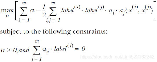
The solution to a quadratic programming problem in M variables in general has computational complexity that is O(M3). In going to the dual formulation we have turned the original optimization problem, which involved minimizing (7.6) over M variables, into the dual problem (7.10), which has N variables. For a fixed set of basis functions whose number M(number of features) is smaller than the number N of data points, the move to the dual problem appears disadvantageous. However, it allows the model to be reformulated using kernels, and so the maximum margin classifier can be applied efficiently to feature spaces whose dimensionality (M*N)exceeds the number(N) of data points, including infinite feature spaces.
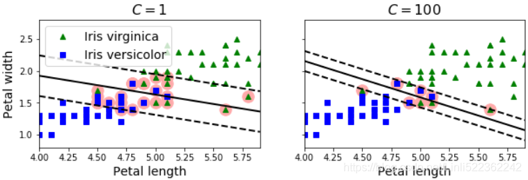
In Scikit-Learn’s SVM classes, you can control this balance using the C hyperparameter: a smaller C value leads to a wider street but more margin violations. Figure 5-4 shows the decision boundaries and margins of two soft margin SVM classifiers on a nonlinearly separable dataset. On the left, using a high C value the classifier makes fewer margin violations but ends up with a smaller margin. On the right, using a low C value the margin is much larger, but many instances end up on the street. However, it seems likely that the second classifier will generalize better: in fact even on this training set it makes fewer prediction errors, since most of the margin violations are actually on the correct side of the decision boundary.
soft margin classification.
This is great, but it makes one assumption: the data is 100% linearly separable(we can use hard margin classification). We know by now that our data is hardly ever that clean. With the introduction of something called slack variables ![]() , we can allow some data points to be on the wrong side of the decision boundary. Our optimization goal stays the same, but we now have a new set of constraints:
, we can allow some data points to be on the wrong side of the decision boundary. Our optimization goal stays the same, but we now have a new set of constraints: 
The constant C controls weighting between our goal of making the margin large and ensuring that most of the data points have a functional margin of at least 1.0. The constant C is an argument to our optimization code that we can tune and get different results. Once we solve for our alphas, we can write the separating hyperplane in terms of these alphas. That part is straightforward. The majority of the work in SVMs is finding the alphas.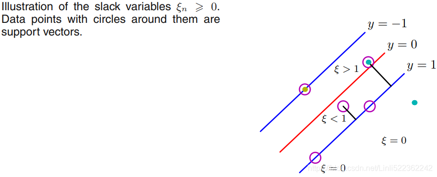
with ξn > 1 will be misclassified. The exact classification constraints (7.5: ![]() ) are then replaced with
) are then replaced with ![]()
![]()
in which the slack variables are constrained to satisfy ![]() . Data points for which ξn = 0 are correctly classified and are either on the margin or on the correct side of the margin. Points for which
. Data points for which ξn = 0 are correctly classified and are either on the margin or on the correct side of the margin. Points for which ![]() lie inside the margin, but on the correct side of the decision boundary, and those data points for which ξn > 1 lie on the wrong side of the decision boundary and are misclassified, as illustrated in Figure 7.3. This is sometimes described as relaxing the hard margin constraint to give a soft margin and allows some of the training set data points to be misclassified. Note that while slack variables allow for overlapping class distributions, this framework is still sensitive to outliers because the penalty for misclassification increases linearly with ξ.
lie inside the margin, but on the correct side of the decision boundary, and those data points for which ξn > 1 lie on the wrong side of the decision boundary and are misclassified, as illustrated in Figure 7.3. This is sometimes described as relaxing the hard margin constraint to give a soft margin and allows some of the training set data points to be misclassified. Note that while slack variables allow for overlapping class distributions, this framework is still sensitive to outliers because the penalty for misclassification increases linearly with ξ.
Our goal is now to maximize the margin while softly penalizing points that lie on the wrong side of the margin boundary. We therefore minimize 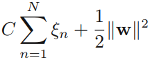
![]()
where the parameter C > 0 controls the trade-off between the slack variable penalty and the margin. Because any point that is misclassified has ξn > 1, it follows that ![]() is an upper bound on the number of misclassified points. The parameter C is therefore analogous相似的 to (the inverse of) a regularization coefficient because it controls the trade-off between minimizing training errors and controlling model complexity. In the limit C → ∞, we will recover the earlier support vector machine for separable data.
is an upper bound on the number of misclassified points. The parameter C is therefore analogous相似的 to (the inverse of) a regularization coefficient because it controls the trade-off between minimizing training errors and controlling model complexity. In the limit C → ∞, we will recover the earlier support vector machine for separable data.
We now wish to minimize (7.21) subject to the constraints (7.20) together with![]() . The corresponding Lagrangian is given by
. The corresponding Lagrangian is given by 
where {![]() 0} and {
0} and {![]() 0} are Lagrange multipliers. The corresponding set of KKT conditions are given by
0} are Lagrange multipliers. The corresponding set of KKT conditions are given by where n = 1,...,N.
We now optimize out w, b, and {ξn} making use of the definition (7.1 ![]() ) of y(x) to give
) of y(x) to give
Using these results to eliminate w, b, and {ξn} from the Lagrangian, we obtain the dual Lagrangian in the form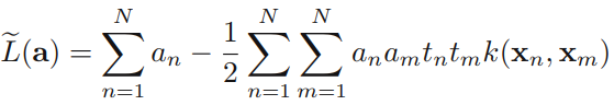
which is identical to the separable case(7.10), except that the constraints are somewhat different. To see what these constraints are, we note that ![]() is required because these are Lagrange multipliers. Furthermore, (7.31) together with
is required because these are Lagrange multipliers. Furthermore, (7.31) together with ![]() implies an C. We therefore have to minimize (7.32) with respect to the dual variables {an} subject to
implies an C. We therefore have to minimize (7.32) with respect to the dual variables {an} subject to
Hinge损失函数
对线性SVM分类器来说,方法之一是使用梯度下降,使从原始问题导出的成本函数最小化。线性SVM分类器cost function成本函数:![]()
成本函数中的第一项会推动模型得到一个较小的权重向量w,从而使间隔更大。
第二项则计算全部的间隔违例。如果没有一个示例位于街道之上,并且都在街道正确的一边,那么这个实例的间隔违例为0;如不然,则该实例的违例大小与其到街道正确一边的距离成正比。所以将这个项最小化,能够保证模型使间隔违例尽可能小,也尽可能少。
函数![]() 被称为hinge损失函数(如下图所示)。其中,t为目标值 class label(-1或+1),y是分类器输出的预测值
被称为hinge损失函数(如下图所示)。其中,t为目标值 class label(-1或+1),y是分类器输出的预测值 ![]() ,并不直接是类标签。其含义为,当t和y的符号相同时(表示y预测正确)并且|y|≥1时,hinge loss为0;当t和y的符号相反时,hinge loss随着y的增大线性增大。
,并不直接是类标签。其含义为,当t和y的符号相同时(表示y预测正确)并且|y|≥1时,hinge loss为0;当t和y的符号相反时,hinge loss随着y的增大线性增大。
Hinge loss用于最大间隔(maximum-margin)分类,其中最有代表性的就是支持向量机SVM。
Hinge函数的标准形式:![]()
(与上面统一的形式:![]() )
)

scaler = StandardScaler()
svm_clf1 = LinearSVC( C=1, loss="hinge", random_state=42 )
svm_clf2 = LinearSVC( C=100, loss="hinge", random_state=42 )

scaled_svm_clf1 = Pipeline([
    ("scaler", scaler),
    ("linear_svc", svm_clf1),
])
scaled_svm_clf2 = Pipeline([
    ("scaler", scaler),
    ("linear_svc", svm_clf2),
])

scaled_svm_clf1.fit(X,y)
scaled_svm_clf2.fit(X,y)
# Bad models
x0 = np.linspace(0, 5.5, 200)
pred_1 = 5*x0 - 20
pred_2 = x0 - 1.8
pred_3 = 0.1 * x0 + 0.5

def plot_svc_decision_boundary(svm_clf, xmin, xmax):
    w = svm_clf.coef_[0] #array([1.29411744, 0.82352928])
    b = svm_clf.intercept_[0] #-3.78823471

    # At the decision boundary, w0*x0 + w1*x1 + b = 0 ==> x1 == -w0/w1*x0 -b/w1
    x0 = np.linspace(xmin, xmax, 200)
    decision_boundary = -w[0]/w[1] *x0 - b/w[1] #x1 #get the separating hyperplane

    #upper-support hyperplane: w0*x0 + w1*x1 + b=1
    #lower-suppert hyperplane: w0*x0 + w1*x1 + b=-1
    #svm_clf.support_vectors_
    #array([[1.9, 0.4],   #lower-support vector
    #       [3. , 1.1]])  #upper-support vector
    margin = 1/w[1] #vertical move
    gutter_up = decision_boundary + margin          #-w[0]/w[1]*x0 -b/w[1] +1/w[1]
    #gutter_up = -w[0]/w[1] *x0 + (svm_clf.support_vectors_[1][1] -(-w[0]/w[1]*svm_clf.support_vectors_[1][0]))
    gutter_down = decision_boundary - margin         #-w[0]/w[1]*x0 -b/w[1] -1/w[1]
    #gutter_down = -w[0]/w[1] *x0 + (svm_clf.support_vectors_[0][1] -(-w[0]/w[1]*svm_clf.support_vectors_[0][0]))
    svs = svm_clf.support_vectors_ #the instances(or the points) located on the edge of the street(called large margin)
    plt.scatter(svs[:,0], svs[:,1], s=180, facecolor='#FFAAAA')
    plt.plot(x0, decision_boundary, "k-", linewidth=2)
    plt.plot(x0, gutter_up, "b--", linewidth=2)
    plt.plot(x0, gutter_down, "k--", linewidth=2)


#As we known as that after doing StandardScaler() then doing linear_svc, the
#new hyperplane has been Offset (the original without doing StandardScaler() prior to linear_svc);
#and here we want to use original dataset so we have to do following processes

#Convert to unscaled parameters
#the seperating hyperplane wx+b
#the seperating hyperplane wx+b=0 means the distance of the points on the seperating
#hyperplane to the seperating hyperplane is equal to 0

#After doing StandardScare,the seperating hyperplane wx+b=0 --offset-->
# w*(x-mean)/scale+b=0 --> w*x/scale +b- w*mean/scale =0
# new w1=w/scale, new b1=b-w*mean/scale

#note: the original decision_function: wx+b
#      the new decision_function: w*(x-mean)/scale+b offset (-mean)/scale

#decision_function: represents the distance from the parameter instance(including some data points) to the separating hyperplane represented by each class
#-scaler.mean_/scaler.scale_ to offset the original separating hyperplane of datapoints
b1 = svm_clf1.decision_function([ -scaler.mean_/scaler.scale_ ])
b2 = svm_clf2.decision_function([ -scaler.mean_/scaler.scale_ ])
w1 = svm_clf1.coef_[0] / scaler.scale_
w2 = svm_clf2.coef_[0] / scaler.scale_
svm_clf1.intercept_ = np.array([b1]) #######new intercept
svm_clf2.intercept_ = np.array([b2]) #######
svm_clf1.coef_ = np.array([w1])      #######new coefficients
svm_clf2.coef_ = np.array([w2])      #######

# Find support vectors (LinearSVC does not do this automatically) of soft margin classification
t = y*2 -1                 #hpyerplane: X.dot(W)+b=0
support_vectors_idx1 = ( t*(X.dot(w1)+b1)<1 ).ravel() #X.dot(w)+b=1 called support hyperplane
support_vectors_idx2 = ( t*(X.dot(w2)+b2)<1 ).ravel() #do selection by True/False
svm_clf1.support_vectors_ = X[support_vectors_idx1] #circled data points
svm_clf2.support_vectors_ = X[support_vectors_idx2]


fig,axes = plt.subplots( ncols=2, figsize=(10,2.7), sharey=True )

plt.sca(axes[0])
plt.plot( X[:,0][y==1], X[:,1][y==1], "g^", label="Iris virginica" )
plt.plot( X[:,0][y==0], X[:,1][y==0], "bs", label="Iris versicolor" )
plot_svc_decision_boundary( svm_clf1, 4, 5.9)
plt.xlabel("Petal length", fontsize=14)
plt.ylabel("Petal width", fontsize=14)
plt.legend( loc="upper left", fontsize=14 )
plt.title( "$C= {}$".format(svm_clf1.C), fontsize=16 )
plt.axis([4,5.9, 0.8,2.8])

plt.sca(axes[1])
plt.plot( X[:,0][y==1], X[:,1][y==1], "g^" )
plt.plot( X[:,0][y==0], X[:,1][y==0], "bs")
plot_svc_decision_boundary(svm_clf2, 4,5.99)
plt.xlabel("Petal length", fontsize=14)
plt.title( "$C= {}$".format(svm_clf2.C), fontsize=16 )
plt.axis([4,5.9, 0.8,2.8])
plt.show()
Figure 5-4. Fewer margin violations versus large margin
#########################################################################
TIP
If your SVM model is overfitting, you can try regularizing it by reducing C.
#########################################################################
########################################extral for understanding decision function
#decision function: represents the distance from the parameter instance[ [3,3],[4,3],[1,1] ] or called sample points
#to the hyperplane represented by each class
X = np.array( [[3,3],[4,3],[1,1]] )
Y = np.array([1,1,-1]) #labels
if we known the separating hyperplane ![]() , we can use decision_function() to get the distance
, we can use decision_function() to get the distance
[ 1. , 1.5, -1. ] to the separating hyperplane for each instances in ( [3,3],[4,3],[1,1] )
import numpy as np
import matplotlib.pyplot as plt
from sklearn import svm

# we create 40 separable points
np.random.seed(0)

X = np.array([[3,3],[4,3],[1,1]])
Y = np.array([1,1,-1])

# fit the model
clf = svm.SVC(kernel='linear')
clf.fit(X, Y)

# get the separating hyperplane
w = clf.coef_[0]
print("w[0]:",w[0])
print("w[1]:",w[1])
print("intercept:",clf.intercept_[0])
print("The separating hyperplane: ", w[0] ,"x1+" , w[1],"x2+" , clf.intercept_[0] )

a = -w[0] / w[1]
xx = np.linspace(-5, 5)
yy = a * xx - (clf.intercept_[0]) / w[1]

# plot the parallels to the separating hyperplane that pass through the
# support vectors
b = clf.support_vectors_[0]
yy_down = a * xx + (b[1] - a * b[0])
b = clf.support_vectors_[-1]
yy_up = a * xx + (b[1] - a * b[0])

# plot the line, the points, and the nearest vectors to the plane
plt.plot(xx, yy, 'k-')
plt.plot(xx, yy_down, 'k--')
plt.plot(xx, yy_up, 'k--')

plt.scatter(clf.support_vectors_[:, 0], clf.support_vectors_[:, 1],
            s=80, facecolor='#FFAAAA')
plt.scatter(X[:, 0], X[:, 1], c=Y, cmap=plt.cm.Paired)

plt.axis('tight')
plt.xlabel("x1", fontsize=14)
plt.ylabel("x2", fontsize=14, rotation=0)
plt.show()

print(clf.decision_function(X))
#########################################################################
The following Scikit-Learn code loads the iris dataset, scales the features, and then trains a linear SVM model (using the LinearSVC class with C = 0.1 and the hinge loss function, described shortly) to detect Iris-Virginica flowers. The resulting model is represented on the right of Figure 5-4.
import numpy as np
from sklearn import datasets
from sklearn.pipeline import Pipeline
from sklearn.preprocessing import StandardScaler
from sklearn.svm import LinearSVC

iris = datasets.load_iris()
X = iris["data"][:,(2,3)] #petal length, petal width
y = ( iris["target"]==2 ).astype(np.float64) #Iris virginica

scaler = StandardScaler()
svm_clf = Pipeline([
    ("scaler", scaler ),
    ("linear_svc", LinearSVC(C=1, loss="hinge", random_state=42))
])

svm_clf.fit(X,y)
svm_clf.predict([ [5.5, 1.7] ]) # 1:Iris versicolor![]()
#################################
NOTE
Unlike Logistic Regression classifiers, SVM classifiers do not output probabilities for each class.
#################################
Alternatively, you could use the SVC class, using SVC(kernel="linear", C=1), but it is much slower, especially with large training sets, so it is not recommended. Another option is to use the SGDClassifier class, with SGDClassifier(loss="hinge", alpha=1/(m*C)). This applies regular Stochastic Gradient Descent (see
https://blog.csdn.net/Linli522362242/article/details/104070847) to train a linear SVM classifier. It does not converge as fast as the LinearSVC class, but it can be useful to handle huge datasets that do not fit in memory (out-of-core training), or to handle online classification tasks.
#################################
TIP
The LinearSVC class regularizes the bias term, so you should center the training set first by subtracting its mean. This is
automatic if you scale the data using the StandardScaler. Moreover, make sure you set the loss hyperparameter to "hinge", as it is not the default value. Finally, for better performance you should set the dual hyperparameter to False, unless there are more features than training instances (we will discuss duality later
#################################
Nonlinear SVM Classification
Although linear SVM classifiers are efficient and work surprisingly well in many cases, many datasets are not even close to being linearly separable. One approach to handling nonlinear datasets is to add more features, such as polynomial features (https://blog.csdn.net/Linli522362242/article/details/104005906); in some cases this can result in a linearly separable dataset. Consider the left plot in Figure 5-5: it represents a simple dataset with just one feature x1. This dataset is not linearly separable, as you can see. But if you add a second feature x2 = ![]() , the resulting 2D dataset is perfectly linearly separable.
, the resulting 2D dataset is perfectly linearly separable.
X1D = np.linspace(-4,4,9).reshape(-1,1)
X2D = np.c_[X1D, X1D**2]
y = np.array([0,0,1,1,1,1,1,0,0]) #labels

plt.figure(figsize=(10,3))

plt.subplot(121)
plt.grid(True, which="both")
plt.axhline(y=0, color='k')
plt.plot(X1D[:,0][y==0], np.zeros(4), "bs")
plt.plot(X1D[:,0][y==1], np.zeros(5), "g^")
plt.gca().get_yaxis().set_ticks([])#########remove ticks on yaxis
plt.xlabel(r"$x_1$", fontsize=20)
plt.axis([-4.5, 4.5, -0.2, 0.2])

plt.subplot(122)
plt.grid(True, which="both")
plt.axhline(y=0, color="k")
plt.axvline(x=0, color="k")
plt.plot(X2D[:,0][y==0], X2D[:,1][y==0], "bs")
plt.plot(X2D[:,0][y==1], X2D[:,1][y==1], "g^")
plt.xlabel(r"$x_1$", fontsize=20)
plt.ylabel(r"$x_2$   ", fontsize=20, rotation=0)
plt.gca().get_yaxis().set_ticks([0,4,8,12,16])
plt.plot([-4.5, 4.5], [6.5, 6.5], "r--", linewidth=3)
plt.axis([-4.5, 4.5, -1, 17])

#subplots_adjust(left=None, bottom=None, right=None, top=None, wspace=None, hspace=None)
plt.subplots_adjust(right=1.5)
plt.show()
Figure 5-5. Adding features to make a dataset linearly separable

############################################### extral materials
subplots_adjust(left=None, bottom=None, right=None, top=None, wspace=None, hspace=None)
    Tune the subplot layout.

    The parameter meanings (and suggested defaults) are::

      left = 0.125  # the left side of the subplots of the figure
      right = 0.9   # the right side of the subplots of the figure
      bottom = 0.1  # the bottom of the subplots of the figure
      top = 0.9     # the top of the subplots of the figure
      wspace = 0.2  # the amount of width reserved for space between subplots,
                    # expressed as a fraction of the average axis width
      hspace = 0.2  # the amount of height reserved for space between subplots,
                    # expressed as a fraction of the average axis height

    The actual defaults are controlled by the rc file

###############################################
To implement this idea using Scikit-Learn, you can create a Pipeline containing a PolynomialFeatures transformer (discussed in “Polynomial Regression” on https://blog.csdn.net/Linli522362242/article/details/104070847), followed by a StandardScaler and a LinearSVC. Let’s test this on the moons dataset (see Figure 5-6):
from sklearn.datasets import make_moons
      # make_moons: Make two interleaving half circles
      #http://lijiancheng0614.github.io/scikit-learn/modules/generated/sklearn.datasets.make_moons.html
X,y = make_moons(n_samples=100, noise=0, random_state=42)
                                #######
def plot_dataset(X,y, axes):
    plt.plot(X[:,0][y==0], X[:,1][y==0], "bs")
    plt.plot(X[:,0][y==1], X[:,1][y==1], "g^")
    plt.axis(axes)
    plt.grid(True, which="both")
    plt.xlabel(r"$x_1$", fontsize=20)
    plt.ylabel(r"$x_2$", fontsize=20, rotation=0)

plot_dataset(X,y, [-1.5,2.5,-1,1.5])
plt.show()
from sklearn.datasets import make_moons
      # make_moons: Make two interleaving half circles
      #http://lijiancheng0614.github.io/scikit-learn/modules/generated/sklearn.datasets.make_moons.html
X,y = make_moons(n_samples=100, noise=0.15, random_state=42)
                                ##########
def plot_dataset(X,y, axes):
    plt.plot(X[:,0][y==0], X[:,1][y==0], "bs")
    plt.plot(X[:,0][y==1], X[:,1][y==1], "g^")
    plt.axis(axes)
    plt.grid(True, which="both")
    plt.xlabel(r"$x_1$", fontsize=20)
    plt.ylabel(r"$x_2$", fontsize=20, rotation=0)

plot_dataset(X,y, [-1.5,2.5,-1,1.5])
plt.show()
from sklearn.datasets import make_moons
from sklearn.pipeline import Pipeline
from sklearn.preprocessing import PolynomialFeatures

polynomial_svm_clf = Pipeline([
    ("poly_features", PolynomialFeatures(degree=3)),
    ("scaler", StandardScaler()),
    ("svm_clf", LinearSVC(C=10, loss="hinge", random_state=42))
])
polynomial_svm_clf.fit(X,y)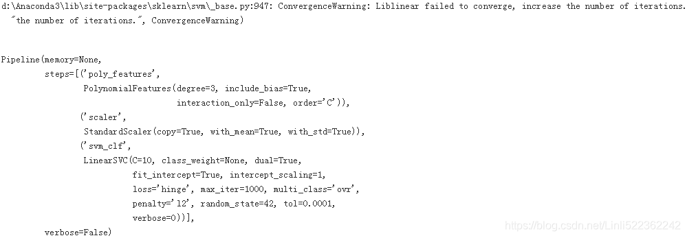
def plot_predictions(clf, axes):
    x0s = np.linspace(axes[0], axes[1], 100)
    x1s = np.linspace(axes[2], axes[3], 100)
    x0, x1 = np.meshgrid(x0s, x1s)
    X = np.c_[x0.ravel(), x1.ravel()]
    y_pred = clf.predict(X).reshape(x0.shape)
    y_decision = clf.decision_function(X).reshape(x0.shape)
    plt.contourf(x0,x1, y_pred, cmap=plt.cm.brg, alpha=0.2)
    plt.contourf(x0,x1,y_decision,cmap=plt.cm.brg, alpha=0.1)

plot_predictions(polynomial_svm_clf, [-1.5,2.5, -1,1.5])
plot_dataset(X,y,[-1.5,2.5, -1,1.5])
plt.title("Figure 5-6. Linear SVM classifier using polynomial features")
plt.show()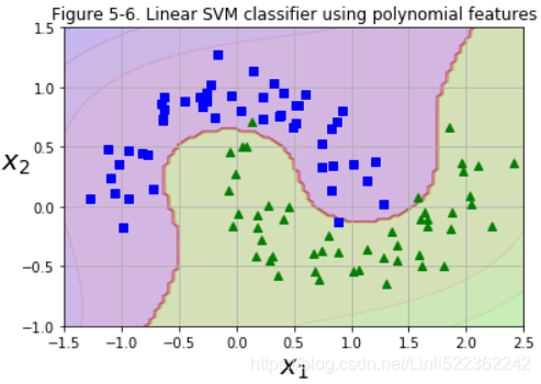
Polynomial Kernel
Adding polynomial features is simple to implement and can work great with all sorts of Machine Learning algorithms (not just SVMs), but at a low polynomial degree it cannot deal with very complex datasets, and with a high polynomial degree it creates a huge number of features, making the model too slow.
Fortunately, when using SVMs you can apply an almost miraculous神奇的 mathematical technique called the kernel trick (it is explained in a moment). It makes it possible to get the same result as if you added many polynomial features, even with very highdegree polynomials, without actually having to add them. So there is no combinatorial explosion组合爆炸 of the number of features since you don’t actually add any features. This trick is implemented by the SVC class. Let’s test it on the moons dataset:
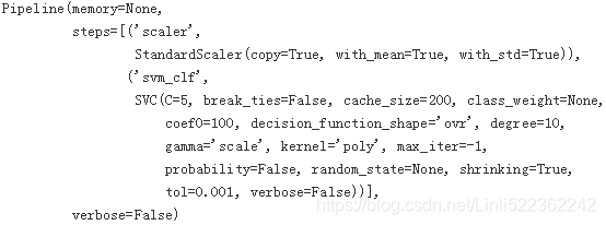
This code trains an SVM classifier using a 3rd-degree polynomial kernel. It is represented on the left of Figure 5-7. On the right is another SVM classifier using a 10th-degree polynomial kernel. Obviously, if your model is overfitting, you might want to reduce the polynomial degree. Conversely, if it is underfitting, you can try increasing it. The hyperparameter coef0 controls how much the model is influenced by high-degree polynomials versus low-degree polynomials.
https://blog.csdn.net/Linli522362242/article/details/104070847![]() or
or ![]()
By increasing the value of the hyperparameter ![]() (the following uses
(the following uses  ), we increase the regularization strength(for tackling the problem of overfitting) and shrink the weights of our model(or reduce the value of wj or bj) since we want to make the function attain the minimum( including ). Note sometimes the value of wj or theta_i is not steady or maybe too large. If α is very large, then all weights end up very close to zero
 |  C : float, optional (default=1.0)
 |      Regularization parameter. The strength of the regularization is
 |      inversely proportional to C. Must be strictly positive. The penalty
 |      is a squared l2 penalty.
from sklearn.svm import SVC
poly_kernel_svm_clf = Pipeline([
("scaler", StandardScaler()),
("svm_clf", SVC(kernel="poly", degree=3, coef0=1, C=5)),
])
#X,y = make_moons(n_samples=100, noise=0.15, random_state=42)
poly_kernel_svm_clf.fit(X,y)
from sklearn.svm import SVC

poly100_kernel_svm_clf = Pipeline([
    ("scaler", StandardScaler()),
    ("svm_clf", SVC(kernel="poly", degree=10, coef0=100, C=5))
])

poly100_kernel_svm_clf.fit(X,y)