详细代码参考:github
Logistics回归
实例:
建立Logistics模型,根据学生的两门考试成绩,判断该学生是否能被大学录取。
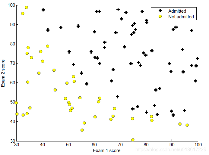
1.可视化数据
解决问题前,不妨先看下数据是怎么分布的,训练数据为100位同学两门课的成绩和录取结果,·shape为(100 ,3),根据录取结果,录取的“+”表示,不能录取的“·”表示,根据图中分布,大致存在一条直线能够将两部分数据进行分类,接下来就去求解这条直线。
参考代码:
def plottingData(self):
	y1_index = np.where(self.y == 1.0)
	x1 = self.x[y1_index[0]]
	y0_index = np.where(self.y == 0.0)
	x0 = self.x[y0_index[0]]
	plt.scatter(x1[:, 0], x1[:, 1], marker='+', color='k')
	plt.scatter(x0[:, 0], x0[:, 1], color='y')
	plt.xlabel('Exam 1 score')
	plt.ylabel('Exam 2 score')
2.Sigmoid函数
我们暂且只考虑二分类问题,根据sigmoid函数的结果,当结果大于0.5时,判断为1,结果小于0.5时,判断为0.
公式:
参考代码:(比较简单,考虑矩阵也要用)
def sigmoid(self, z):
	return 1 / (1 + np.exp(-z))

def predict0_1(self, theta):
	self.p = np.zeros((100, 1))
	self.p = self.sigmoid(self.x_plus1.dot(np.array(theta).reshape(3, 1)))
	for i in range(len(self.p)):
		if self.p[i] < 0.5:
			self.p[i] = 0
		else:
			self.p[i] = 1
		i += 1
	return self.p
3.损失函数和梯度
逻辑回归的损失函数分为两部分,将y=0 和y=1的部分结合在一起,整体写出来如下。尤其注意矩阵相乘的时候维度匹配的问题,我经常在本子上把维度计算下,如:x的shape(100, 3),theta(3, 1)结果shape肯定是(100,1),如果程序报维度错误,也能很快的发现哪里需要修改。
对theta求偏导数:
参考代码:
def costFunction(self, theta):
	m = len(self.y)
	J = np.sum(-np.dot(self.y.T, np.log(self.sigmoid(self.x_plus1.dot(theta))))\
		-np.dot((1-self.y).T, np.log(1-self.sigmoid(self.x_plus1.dot(theta)))), axis=0) / m
	return J

def gradient(self, theta):
	m = len(self.y)
	theta = theta.reshape((3, 1))
	grad = np.dot(self.x_plus1.T, (self.sigmoid(self.x_plus1.dot(theta))-self.y)) / m
	return grad
4.求解最优的theta
如果利用梯度下降的方法求解比较费时间,有大神已经尝试,在这里就不展开了,原Octave程序中使用了fminunc函数,经查找,发现了一篇大神的博客:Python fminunc 的替代方法,利用scipy.optimize中的minimize函数,详细内容还是看大神的博客,尤其注意result = op.minimize(fun=costFunction, x0=initial_theta, args=(X, Y), method='TNC', jac=gradient)中x0的维度,应该是(n, )。
参考代码:
def fminunc(self):  # costFunction需要几个参数就传几个,本例中只有一个theta,固x0,也可以利用args=()
	optiTheta = op.minimize(fun=self.costFunction, x0=self.init_theta, method='TNC', jac=self.gradient)
	return optiTheta  # dict
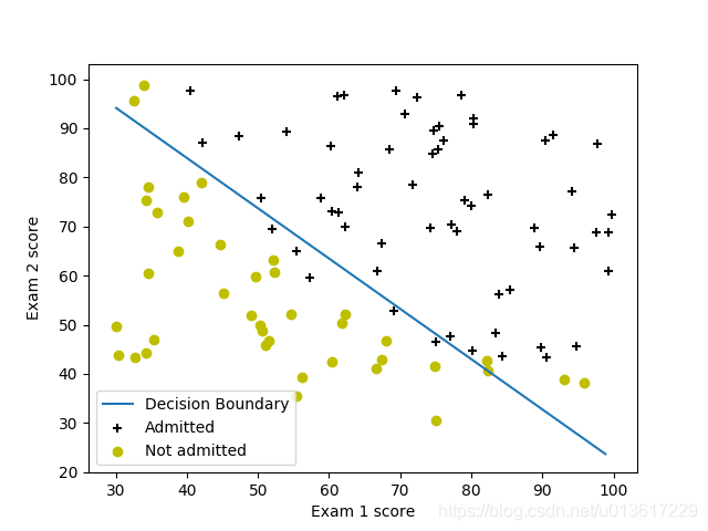
5.绘制拟合曲线
由于特征为两个,这里采取简单的两点绘制直线的方法。
参考代码:
def plotRegLine(self):  # 两点确定一条直线
	self.opti_theta = self.fminunc()['x']
	plot_x = [np.min(self.x[:, 0]), np.max(self.x[:, 1])]  # [A, B]
	plot_y = [-(self.opti_theta[0] + self.opti_theta[1]*x)/self.opti_theta[2] for x in plot_x]  # [A, B]
	self.plottingData()
	plt.plot(plot_x, plot_y)
	plt.legend(['Decision Boundary', 'Admitted', 'Not admitted'])
	plt.show()
5.准确率
利用求得的最优解theta反过来求解x的分类,和y本身做对比,求解准确率,得到结果为89%,这里没有单独设置测试集,也可以随机80%的数据作为训练集,剩余20%用作测试集。
参考代码::
def predictAndAccuracies(self):
	prob = self.sigmoid(np.array(self.opti_theta).reshape(1, 3).dot(np.array([[1], [45], [85]])))
	print('For a student with scores with 45 and 85, we predict an admission probability of %f' % prob)
	accuracy = np.mean(self.predict0_1(self.opti_theta) == self.y)*100
	print('Train Accuracy: %f' % accuracy)