How to do Semantic Segmentation using Deep learning(如何使用深度学习进行语义分割)

This article is a comprehensive overview including a step-by-step guide to implement a deep learning image segmentation model.

update: We just launched a new product: [Nanonets Object Detection APIs

](https://nanonets.com/object-detection-api/?utm_source=medium.com_Semantic_Segmentation&utm_medium=blog&utm_campaign=semantic_segmentation)

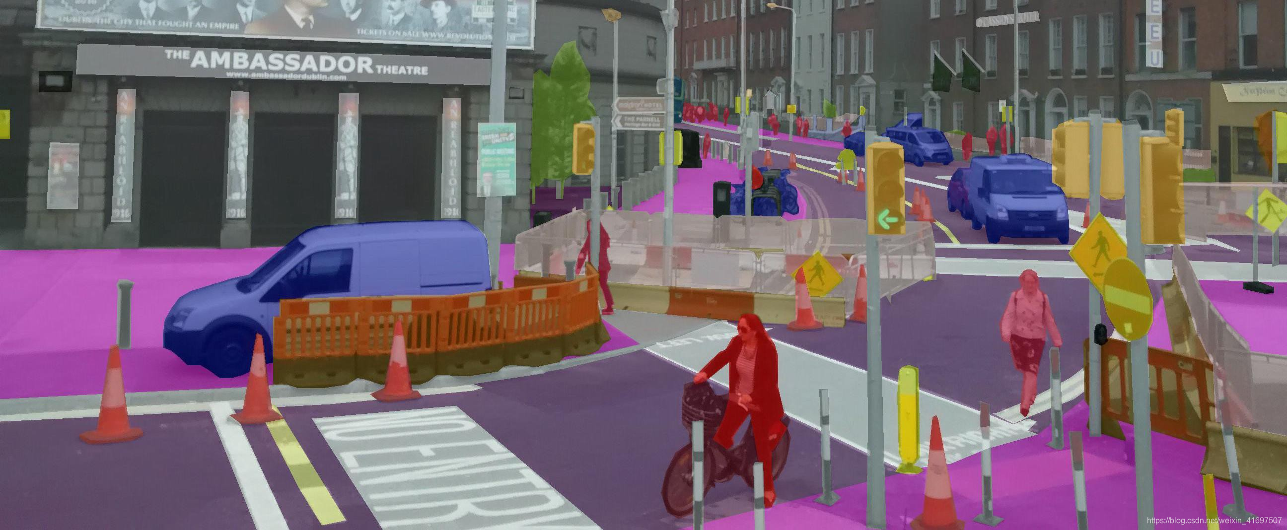
Deeplab Image Semantic Segmentation Network (Source: https://sthalles.github.io/deep_segmentation_network/)

如今，语义分割是计算机视觉领域的关键问题之一。 纵观全局，语义分割是为完整场景理解铺平道路的高级任务之一。 场景理解作为核心计算机视觉问题的重要性突出表现在越来越多的应用程序通过从图像推断知识而滋养。 其中一些应用包括自动驾驶车辆，人机交互，虚拟现实等。随着近年来深度学习的普及，许多语义分段问题正在使用深层架构解决，最常见的是卷积神经网络，超越其他方法 在准确性和效率方面有很大的差距。

What is Semantic Segmentation?

语义分割是从粗略推理到精细推理的自然步骤：

• 原点可以位于分类，包括对整个输入进行预测。
• 下一步是本地化/检测，它不仅提供类，还提供有关这些类的空间位置的附加信息。
• 最后，语义分割通过进行密集预测推断每个像素的标签来实现细粒度推理，从而每个像素都用其封闭对象矿石区域的类别进行标记。
  

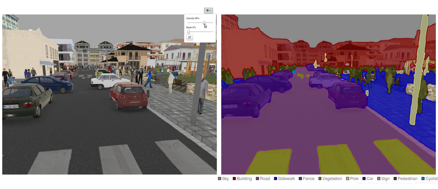
An example of semantic segmentation (Source: https://blog.goodaudience.com/using-convolutional-neural-networks-for-image-segmentation-a-quick-intro-75bd68779225)

值得回顾一些对计算机视觉领域做出重大贡献的标准深度网络，因为它们经常被用作语义分割系统的基础：

AlexNet：多伦多开创性的深度CNN赢得了2012年ImageNet竞赛，测试精度为84.6％。它由5个卷积层组成，最大池化，ReLU为非线性，3个完全卷积层和丢失。
VGG-16：这个牛津大学的模型以92.7％的准确率赢得了2013年ImageNet大赛。它使用一堆卷积层，在第一层中具有小的感受野，而不是具有大的感受野的少数层。
GoogLeNet：这个Google的网络赢得了2014年ImageNet竞赛，准确率为93.3％。它由22层和一个新引入的构建块组成，称为初始模块。该模块由网络中的网络层，池化操作，大型卷积层和小型卷积层组成。
ResNet：这款微软的模型以96.4％的准确率赢得了2016年ImageNet大赛。由于其深度（152层）和残余块的引入，它是众所周知的。剩余块通过引入标识跳过连接来解决训练真正深层架构的问题，以便层可以将其输入复制到下一层。

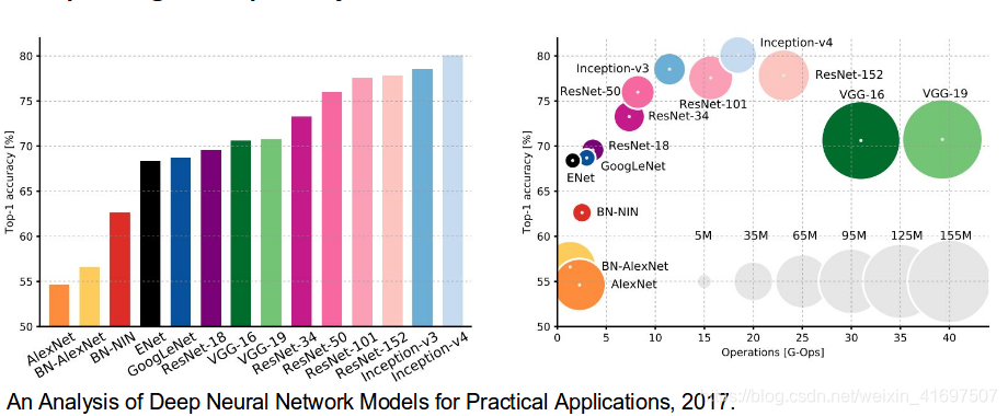
CNN Architectures (Source: https://www.semanticscholar.org/paper/An-Analysis-of-Deep-Neural-Network-Models-for-Canziani-Paszke/28ee688947cf9d31fc48f07a0497cd75200a9485)

What are the existing Semantic Segmentation approaches?

一般的语义分割体系结构可以被广泛地认为是编码器网络，后面是解码器网络：

• 编码器通常是预先训练的分类网络，如VGG / ResNet，后跟解码器网络。
• 解码器的任务是将编码器学习的判别特征（较低分辨率）语义投影到像素空间（较高分辨率）以获得密集分类。

与深度网络的最终结果是唯一重要的分类不同，语义分割不仅需要在像素级别进行区分，而且还需要将在编码器的不同阶段学习的判别特征投影到像素空间上的机制。 不同的方法采用不同的机制作为解码机制的一部分。 让我们探讨三种主要方法：## 1 — Region-Based Semantic Segmentation
The region-based methods generally follow the “segmentation using recognition” pipeline, which first extracts free-form regions from an image and describes them, followed by region-based classification. At test time, the region-based predictions are transformed to pixel predictions, usually by labeling a pixel according to the highest scoring region that contains it.

R-CNN Architecture

R-CNN（具有CNN特征的区域）是基于区域的方法的一个代表性工作。它基于对象检测结果执行语义分割。具体而言，R-CNN首先利用选择性搜索来提取大量的对象提议，然后为每个提议计算CNN特征。最后，它使用类特定的线性SVM对每个区域进行分类。与主要用于图像分类的传统CNN结构相比，R-CNN可以解决更复杂的任务，如物体检测和图像分割，甚至成为这两个领域的重要基础。此外，R-CNN可以构建在任何CNN基准结构之上，例如AlexNet，VGG，GoogLeNet和ResNet。

对于图像分割任务，R-CNN为每个区域提取了两种类型的特征：全区域特征和前景特征，并发现当将它们连接在一起作为区域特征时，它可以带来更好的性能。由于使用高度辨别力的CNN特征，R-CNN实现了显着的性能改进。但是，它也会受到分段任务的一些缺点：

该功能与分段任务不兼容。
该特征不包含足够的空间信息以用于精确的边界生成。
生成基于段的提议需要时间，并且会极大地影响最终的性能。
由于这些瓶颈，最近提出了解决这些问题的研究，包括SDS，Hypercolumns .pdf），Mask R-CNN。

2 — Fully Convolutional Network-Based Semantic Segmentation

最初的完全卷积网络（FCN）学习从像素到像素的映射，而不提取区域提议。 FCN网络管道是传统CNN的扩展。 主要思想是使经典CNN作为输入任意大小的图像。 CNN仅限于特定尺寸输入接受和生成标签的限制来自固定的完全连接的层。 与它们相反，FCN只有卷积和汇集层，使他们能够对任意大小的输入进行预测。

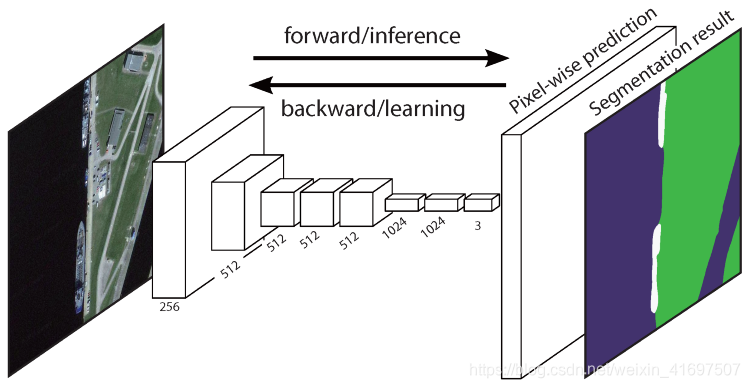
FCN Architecture

该特定FCN中的一个问题是通过传播几个交替的卷积和池化层，输出特征图的分辨率被下采样。 因此，FCN的直接预测通常是低分辨率的，导致相对模糊的对象边界。 已经提出了各种更先进的基于FCN的方法来解决这个问题，包括SegNet，[DeepLab-CRF](https://arxiv.org /pdf/1412.7062.pdf)和Dilated Convolutions。

3 — Weakly Supervised Semantic Segmentation

语义分割中的大多数相关方法依赖于具有逐像素分割掩模的大量图像。 然而，手动注释这些掩模非常耗时，令人沮丧且商业上昂贵。 因此，最近提出了一些弱监督方法，这些方法致力于通过利用带注释的边界框来实现语义分割。

Boxsup Training

例如，Boxsup使用边界框注释作为监督来训练网络并迭代地改进用于语义分割的估计掩模。简单是否将弱监督限制视为输入标签噪声问题，并将递归训练作为去噪策略进行探讨。像素级标签解释了多实例学习框架内的分段任务，并添加了一个额外的层来约束模型，以便为重要像素分配更多权重以进行图像级分类。

用全卷积网络进行语义分割
在本节中，让我们逐步实现最流行的语义分割架构 - 全卷积网络（FCN）。我们将使用Python 3中的TensorFlow库以及其他依赖项（如Numpy和Scipy）来实现它。

在本练习中，我们将使用FCN标记图像中道路的像素。我们将与Kitti Road Dataset一起进行道路/车道检测。这是Udacity的自动驾驶汽车纳米学位课程的简单练习，您可以在GitHub repo中了解更多有关设置的信息。

Kitti Road Dataset Training Sample (Source: http://www.cvlibs.net/datasets/kitti/eval_road_detail.php?result=3748e213cf8e0100b7a26198114b3cdc7caa3aff)

以下是FCN架构的主要功能：

• FCN从VGG16传输知识以执行语义分段。
• 使用1x1卷积将VGG16的完全连接层转换为完全卷积层。该过程以低分辨率产生类存在热图。
• 使用转置卷积（用双线性插值滤波器初始化）完成这些低分辨率语义特征映射的上采样。
• 在每个阶段，通过添加来自VGG16中较低层的较粗但较高分辨率的特征图的特征，进一步细化上采样过程。
• 在每个卷积块之后引入跳过连接，以使后续块从先前合并的特征中提取更抽象的，类显着的特征。

FCN有3个版本（FCN-32，FCN-16，FCN-8）。我们将实施FCN-8，详细步骤如下：

编码器：预训练的VGG16用作编码器。解码器从VGG16的第7层开始。
FCN第8层：VGG16的最后一个完全连接层被1x1卷积取代。
FCN第9层：FCN第8层上采样2次以匹配VGG 16第4层的尺寸，使用带参数的转置卷积：（kernel =（4,4），stride =（2,2），paddding ='same “）。之后，在VGG16的第4层和FCN第9层之间添加了跳过连接。
FCN第10层：FCN第9层上采样2次以匹配VGG16第3层的维度，使用带参数的转置卷积：（kernel =（4,4），stride =（2,2），paddding =‘same’ ）。之后，在VGG 16的第3层和FCN第10层之间添加跳过连接。
FCN Layer-11：FCN Layer-10上采样4次以匹配输入图像大小的尺寸，因此我们使用带参数的转置卷积来获得实际图像并且深度等于类的数量：（kernel =（16,16） ，stride =（8,8），paddding =‘same’）。

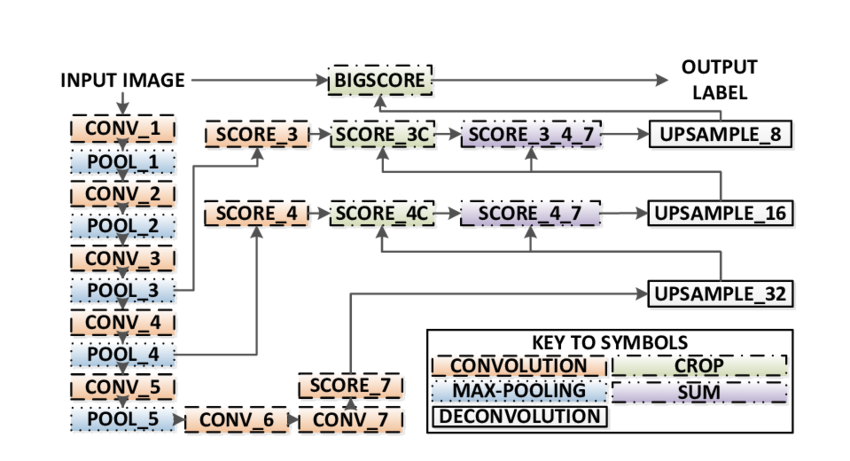
FCN-8 Architecture (Source: https://www.researchgate.net/figure/Illustration-of-the-FCN-8s-network-architecture-as-proposed-in-20-In-our-method-the_fig1_305770331)

Step 1

我们首先将预先训练的VGG-16模型加载到TensorFlow中。 接受TensorFlow会话和VGG文件夹的路径（可下载这里，我们从VGG返回张量元组 模型，包括图像输入，keep_prob（控制丢失率），第3层，第4层和第7层。

def load_vgg(sess, vgg_path):
  
  # load the model and weights
  model = tf.saved_model.loader.load(sess, ['vgg16'], vgg_path)

  # Get Tensors to be returned from graph
  graph = tf.get_default_graph()
  image_input = graph.get_tensor_by_name('image_input:0')
  keep_prob = graph.get_tensor_by_name('keep_prob:0')
  layer3 = graph.get_tensor_by_name('layer3_out:0')
  layer4 = graph.get_tensor_by_name('layer4_out:0')
  layer7 = graph.get_tensor_by_name('layer7_out:0')

  return image_input, keep_prob, layer3, layer4, layer7

Step 2

现在我们专注于使用VGG模型中的张量为FCN创建图层。 给定VGG层输出的张量和要分类的类的数量，我们返回该输出的最后一层的张量。 特别是，我们将1x1卷积应用于编码器层，然后通过跳过连接和上采样将解码器层添加到网络。

def layers(vgg_layer3_out, vgg_layer4_out, vgg_layer7_out, num_classes):
   
    # Use a shorter variable name for simplicity
    layer3, layer4, layer7 = vgg_layer3_out, vgg_layer4_out, vgg_layer7_out

    # Apply 1x1 convolution in place of fully connected layer
    fcn8 = tf.layers.conv2d(layer7, filters=num_classes, kernel_size=1, name="fcn8")

    # Upsample fcn8 with size depth=(4096?) to match size of layer 4 so that we can add skip connection with 4th layer
    fcn9 = tf.layers.conv2d_transpose(fcn8, filters=layer4.get_shape().as_list()[-1],
    kernel_size=4, strides=(2, 2), padding='SAME', name="fcn9")

    # Add a skip connection between current final layer fcn8 and 4th layer
    fcn9_skip_connected = tf.add(fcn9, layer4, name="fcn9_plus_vgg_layer4")

    # Upsample again
    fcn10 = tf.layers.conv2d_transpose(fcn9_skip_connected, filters=layer3.get_shape().as_list()[-1],
    kernel_size=4, strides=(2, 2), padding='SAME', name="fcn10_conv2d")

    # Add skip connection
    fcn10_skip_connected = tf.add(fcn10, layer3, name="fcn10_plus_vgg_layer3")

    # Upsample again
    fcn11 = tf.layers.conv2d_transpose(fcn10_skip_connected, filters=num_classes,
    kernel_size=16, strides=(8, 8), padding='SAME', name="fcn11")

    return fcn11

Step 3

下一步是优化我们的神经网络，即建立TensorFlow损失函数和优化器操作。 这里我们使用交叉熵作为我们的损失函数，使用Adam作为我们的优化算法。

def optimize(nn_last_layer, correct_label, learning_rate, num_classes):
  
  # Reshape 4D tensors to 2D, each row represents a pixel, each column a class
  logits = tf.reshape(nn_last_layer, (-1, num_classes), name="fcn_logits")
  correct_label_reshaped = tf.reshape(correct_label, (-1, num_classes))

  # Calculate distance from actual labels using cross entropy
  cross_entropy = tf.nn.softmax_cross_entropy_with_logits(logits=logits, labels=correct_label_reshaped[:])
  # Take mean for total loss
  loss_op = tf.reduce_mean(cross_entropy, name="fcn_loss")

  # The model implements this operation to find the weights/parameters that would yield correct pixel labels
  train_op = tf.train.AdamOptimizer(learning_rate=learning_rate).minimize(loss_op, name="fcn_train_op")

  return logits, train_op, loss_op

Step 4

这里我们定义train_nn函数，它接受重要的参数，包括历元数，批量大小，损失函数，优化器操作，输入图像的占位符，标签图像，学习率。 对于培训过程，我们还将keep_probability设置为0.5，将learning_rate设置为0.001。 为了跟踪进度，我们还在培训期间打印出损失。

def train_nn(sess, epochs, batch_size, get_batches_fn, train_op,
             cross_entropy_loss, input_image,
             correct_label, keep_prob, learning_rate):

  keep_prob_value = 0.5
  learning_rate_value = 0.001
  for epoch in range(epochs):
      # Create function to get batches
      total_loss = 0
      for X_batch, gt_batch in get_batches_fn(batch_size):

          loss, _ = sess.run([cross_entropy_loss, train_op],
          feed_dict={input_image: X_batch, correct_label: gt_batch,
          keep_prob: keep_prob_value, learning_rate:learning_rate_value})

          total_loss += loss;

      print("EPOCH {} ...".format(epoch + 1))
      print("Loss = {:.3f}".format(total_loss))
      print()

Step 5

最后，是时候训练我们的网了！ 在这个运行函数中，我们首先使用load_vgg，layers和optimize函数构建我们的网络。 然后我们使用train_nn函数训练网络并保存记录的推理数据。

def run():
  
  # Download pretrained vgg model
  helper.maybe_download_pretrained_vgg(data_dir)

  # A function to get batches
  get_batches_fn = helper.gen_batch_function(training_dir, image_shape)
  
  with tf.Session() as session:
        
    # Returns the three layers, keep probability and input layer from the vgg architecture
    image_input, keep_prob, layer3, layer4, layer7 = load_vgg(session, vgg_path)

    # The resulting network architecture from adding a decoder on top of the given vgg model
    model_output = layers(layer3, layer4, layer7, num_classes)

    # Returns the output logits, training operation and cost operation to be used
    # - logits: each row represents a pixel, each column a class
    # - train_op: function used to get the right parameters to the model to correctly label the pixels
    # - cross_entropy_loss: function outputting the cost which we are minimizing, lower cost should yield higher accuracy
    logits, train_op, cross_entropy_loss = optimize(model_output, correct_label, learning_rate, num_classes)
    
    # Initialize all variables
    session.run(tf.global_variables_initializer())
    session.run(tf.local_variables_initializer())

    print("Model build successful, starting training")

    # Train the neural network
    train_nn(session, EPOCHS, BATCH_SIZE, get_batches_fn, 
             train_op, cross_entropy_loss, image_input,
             correct_label, keep_prob, learning_rate)

    # Run the model with the test images and save each painted output image (roads painted green)
    helper.save_inference_samples(runs_dir, data_dir, session, image_shape, logits, keep_prob, image_input)
    
    print("All done!")

关于我们的参数，我们选择epochs = 40，batch_size = 16，num_classes = 2和image_shape =（160,576）。 在进行2次试验，辍学= 0.5和辍学= 0.75后，我们发现第二次试验产生更好的结果，平均损失更好。

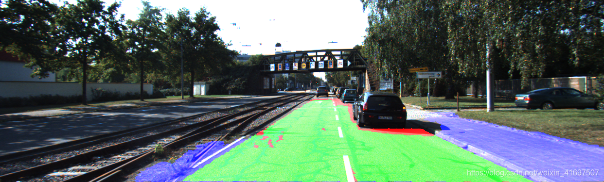
Training Sample Results

To see the full code, check out this link: https://gist.github.com/khanhnamle1994/e2ff59ddca93c0205ac4e566d40b5e88