利用Logistic回归进行分类的主要思想是:根据现有数据对分类边界线建立回归公式,以此进行分类。这里的“回归”一词源于最佳拟合,表示要找到最佳拟合参数集。训练分类器时的做法就是寻找最佳拟合参数,使用的是最优化算法。
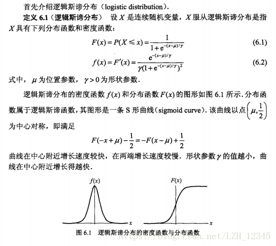
一、 Logistic分布
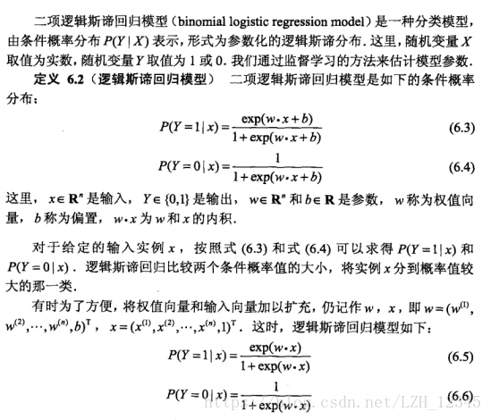
二、 Logistic回归模型(二分类模型)
其中,sigmoid函数:
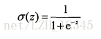
换言之,直接利用sigmoid函数理解二分类Logistic回归模型:
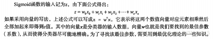
P(Y=1|x)=sigmoid(z);P(Y=0|x)=1-P(Y=1|x)=sigmoid(z)。其中,z的表达式如下:
三、 模型参数估计
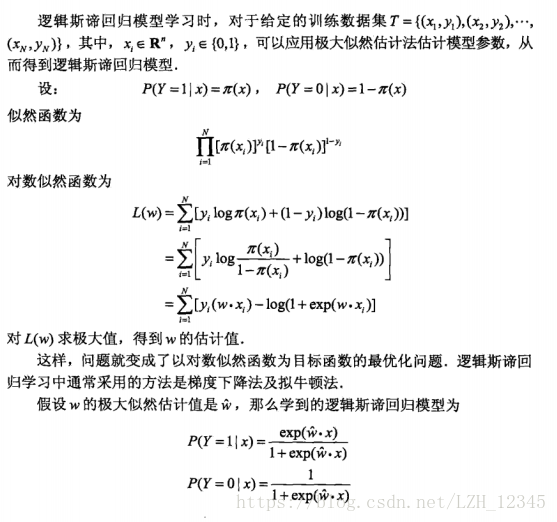
3.1 极大似然函数的方式估计参数:
3.2 梯度上升法估计参数
梯度上升算法用来求函数的最大值,而梯度下降算法用来求函数的最小值。
梯度上升算法迭代公式:
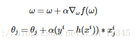
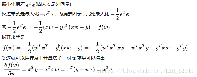
推导第一个:其中e是误差,样本矩阵x,类别标签y,回归系数w,步长a。
梯度上升的目的是最小化误差:
四、基于梯度上升算法估计最佳参数
4.1 代码实现
# -*- coding: utf-8 -*-
"""
Created on Wed Apr 18 19:07:15 2018
file name:logRegres.py
@author: lizihua
"""
import numpy as np
from numpy import exp,mat,shape,ones,array,random
import matplotlib.pyplot as plt
#Logistic回归梯度上升优化算法
#加载数据
#注意,返回的是列表!!!
def loadDataSet():
dataMat = [];labelMat = []
fr = open('testSet.txt')
for line in fr.readlines():
lineArr = line.strip().split()
#添加一列x0=1
dataMat.append([1.0,float(lineArr[0]),float(lineArr[1])])
labelMat.append(int(lineArr[2]))
return dataMat,labelMat
#定义激活函数
def sigmoid(inX):
return 1.0/(1+exp(-inX))
#梯度上升法
def gradAscent(dataMatIn,classLabels):
#将数据转换成矩阵,此时,dataMatIn是list,dataMatrix是矩阵
dataMatrix = mat(dataMatIn)
#将标签数据转换成矩阵,并进行转置(transpose)
labelMat = mat(classLabels).transpose()
#m代表样本数目,n代表特征数目(已加上x0(x0=1)特征)
m,n = shape(dataMatrix)
#初始化:alpha是移动步长,iterNum 是迭代次数,weights是训练好的回归系数
alpha = 0.001
iterNum = 500
weights = ones((n,1))
for k in range(iterNum):
h = sigmoid(dataMatrix*weights)
error = labelMat - h
weights = weights + alpha*dataMatrix.transpose()*error
return weights
#随机梯度上升算法:随机选取一个误分类点来更新回归系数,直至没有误分类点
#随机梯度上升算法:随机选取一个误分类点来更新回归系数,直至没有误分类点
def stocGradAscent0(dataMatrix, classLabels,numIter):
m,n = shape(dataMatrix)
weights = ones(n)
alpha=0.01
weightSet=[]
for j in range(numIter):
for i in range(m):
h = sigmoid(sum(dataMatrix[i]*weights))
error = classLabels[i]-h
#注意:原代码中,输入参数都是列表,列表*小数会报错,所以,将dataMatrix转换成数组array
weights = weights +alpha *error* array(dataMatrix[i])
weightSet.append(weights)
return weights,array(weightSet)
#改进版
def stocGradAscent1(dataMatrix, classLabels,numIter=150):
m,n = shape(dataMatrix)
weights = ones(n)
weightSet=[]
for j in range(numIter):
#python3中range返回的是range对象,后面使用了del方法(list方法),因此,需转成list
dataIndex = list(range(m))
for i in range(m):
#改进2:每次迭代时调整alpha
alpha=4/(1.0+i+j)+0.01
#改进2:随机选取更新
randIndex = int(random.uniform(0,len(dataIndex)))
h = sigmoid(sum(dataMatrix[randIndex]*weights))
error = classLabels[randIndex]-h
#注意:原代码中,输入参数都是列表,列表*小数会报错,所以,将dataMatrix转换成数组array
weights = weights +alpha *error* array(dataMatrix[randIndex])
weightSet.append(weights)
del(dataIndex[randIndex])
return weights,array(weightSet)
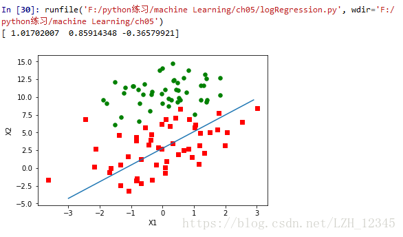
#画出数据集和Logistic回归最佳拟合直线
def plotBestFit(weights):
dataMat,labelMat= loadDataSet()
dataArr = array(dataMat)
m = shape(dataArr)[0]
xcord1 = []; ycord1 = []
xcord0 = []; ycord0 = []
for i in range(m):
if int(labelMat[i])==1:
xcord1.append(dataArr[i,1]); ycord1.append(dataArr[i,2])
else:
xcord0.append(dataArr[i,1]); ycord0.append(dataArr[i,2])
fig = plt.figure()
ax = fig.add_subplot(111)
ax.scatter(xcord1,ycord1,s=30,c='red',marker='s')
ax.scatter(xcord0,ycord0,s=30,c='green')
#绘制拟合直线
x = np.arange(-3.0, 3.0, 0.1) # x取值范围
#weight[1]是1*1的矩阵,x是1*60的矩阵,结果是1*60
#而plot(x,y)要求x和y的shape[0]相同,此时x,y的shape[0]分别是60,1,因此,报错
#错误形式:y = -(weights[0]+weights[1]*x)/weights[2]
#分割线方差设置sigmoid函数为0,即0=w0x0+w1x1+w2x2
y = -(weights[0]+weights[1]*x)/weights[2]
ax.plot(x,y.T)
plt.xlabel('X1'); plt.ylabel('X2')
"""
def plotWeightAndnumIter(weights,numIter):
w0=weight
"""
if __name__=="__main__":
dataArr,labelMat = loadDataSet()
"""
#改进前随机梯度中迭代次数和回归系数之间的关系
weights,weightSet=stocGradAscent0(dataArr,labelMat,2)
numIter = np.arange(0,2*100,1)
plotBestFit(weights)
"""
#改进后迭代次数和回归系数的关系
weights,weightSet=stocGradAscent1(dataArr,labelMat,200)
numIter = np.arange(0,200*100,1)
plotBestFit(weights)
numIter = np.arange(0,200*100,1)
fig1 = plt.figure()
ax1 = fig1.add_subplot(311)
ax1.plot(numIter,weightSet[:,0])
ax2 = fig1.add_subplot(312)
ax2.plot(numIter,weightSet[:,1])
ax3 = fig1.add_subplot(313)
ax3.plot(numIter,weightSet[:,2])
4.2 结果显示
4.2.1 梯度上升算法的结果:
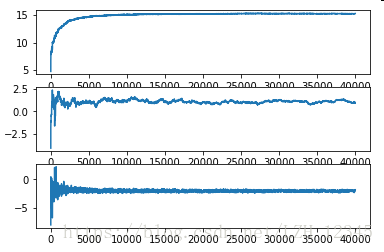
4.2.2 改进前随机梯度上升算法:迭代次数与回归系数的关系:

4.2.3 改进后随机梯度上升算法:迭代次数与回归系数的关系:
五、从疝气病症预测病马的死亡率
代码实现:
# -*- coding: utf-8 -*-
"""
Created on Tue Apr 17 20:58:36 2018
*************************************从疝气病症预测病马的死亡率****************************************
@author: lizihau
"""
from numpy import array,random,exp,shape,ones
import numpy as np
#定义激活函数
def sigmoid(inX):
return 1.0/(1+exp(-inX))
def stocGradAscent1(dataMatrix, classLabels, numIter=150):
m,n = shape(dataMatrix)
weights = ones(n) #initialize to all ones
for j in range(numIter):
dataIndex = list(range(m))
for i in range(m):
alpha = 4/(1.0+j+i)+0.0001 #apha decreases with iteration, does not
randIndex = int(random.uniform(0,len(dataIndex)))#go to 0 because of the constant
h = sigmoid(sum(dataMatrix[randIndex]*weights))
error = classLabels[randIndex] - h
weights = weights + alpha * error * dataMatrix[randIndex]
del(dataIndex[randIndex])
return weights
#分类函数
def classifyVector(inX, weights):
prob = sigmoid(sum(inX*weights))
if prob > 0.5: return 1.0
else: return 0.0
def colicTest():
frTrain = open('horseColicTraining.txt'); frTest = open('horseColicTest.txt')
trainingSet = []; trainingLabels = []
for line in frTrain.readlines():
currLine = line.strip().split('\t')
lineArr =[]
#数据有22列,前21个为特征,最后一个是分类标签
for i in range(21):
lineArr.append(float(currLine[i]))
trainingSet.append(lineArr)
trainingLabels.append(float(currLine[21]))
trainWeights = stocGradAscent1(array(trainingSet), trainingLabels, 1000)
errorCount = 0; numTestVec = 0.0
for line in frTest.readlines():
numTestVec += 1.0
currLine = line.strip().split('\t')
lineArr =[]
for i in range(21):
lineArr.append(float(currLine[i]))
if int(classifyVector(array(lineArr), trainWeights))!= int(currLine[21]):
errorCount += 1
errorRate = (float(errorCount)/numTestVec)
print("测试集错误率: %f" % errorRate)
return errorRate
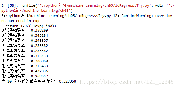
#调用10次colicTest函数,然后求结果的平均值
def multiTest():
numTests = 10; errorSum=0.0
for k in range(numTests):
errorSum += colicTest()
print("第 %d 次迭代的错误率平均值: %f" % (numTests, errorSum/float(numTests)))
if __name__=="__main__":
multiTest()
结构显示: