《机器学习实战》第五章----Logistic回归

Logistic回归

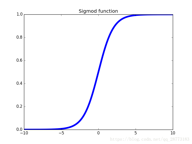
所谓回归,就是给一组数据,构建一个多项式对整个数据进行拟合.建立多项式 $f=\theta_0x_0+\theta_1x_1+\cdots+\theta_nx_n=\theta^TX$ .

sigmod函数

sigmod函数也是一种阶跃函数,为什么经常能看见这个函数在分类问题中经常见到,包括神经网络的激活函数,这是由于S函数在的值域在 $[0,1]$ 之间,当 $x=0$ 时, $y=0.5$ ,很容易理解的一点是,我们可以从概率的角度来说明这个问题,当属于A类的S函数的值大于0.5,则可判断该样本属于A类,则可认为.Sigmod函数的表达式如下:

f (x) = \frac{1}{1 + e^{- x}}

$f(x)=\frac{1}{1+e^{-x}}$
图像如下所示:
这里写图片描述

COST FUNCTION

代价函数的存在是为了训练过程中调整参数的.一般的代价函数用平方误差来表示,并且对于回归问题,这样的代价函数通常是很有用的.假设函数 $h_{\theta}(X)=\frac{1}{1+e^{-\theta^{T}X}}$ ,定义代价函数如下:

J (θ) = \frac{1}{m} \sum_{i = 1}^{m} C o s t (h_{θ} (x^{(i)}), y^{(i)})

$J(\theta)=\frac{1}{m}\sum_{i=1}^m Cost(h_{\theta}(x^{(i)}),y^{(i)})$
其中:

C o s t (h_{θ} (x), y) = {\begin{cases} - l o g (h_{θ} (x)), & if y = 1 \\ - l o g (1 - h_{θ} (x)), & if y = 0 \end{cases}

$Cost(h_{\theta}(x),y)= \begin{cases} -log(h_{\theta}(x)), & \text{if $y=1$ } \\ -log(1-h_{\theta}(x)), & \text{if $y=0$ } \end{cases}$
这里使用

l o g

$log$ 函数也是为了后面梯度算法求导的方便.在一个二分类问题中,我们可以将

y

$y$ 和

1 - y

$1-y$ 作为系数,写成一个统一的代价函数表达式:

C o s t (h_{θ} (x), y) = - y l o g (h_{θ} (x)) - (1 - y) l o g (1 - h_{θ} (x))

$Cost(h_{\theta}(x),y)=-ylog(h_{\theta}(x))-(1-y)log(1-h_{\theta}(x))$
这样得到最终的代价函数

J (θ)

$J(\theta)$ 为:

J (θ) = - \frac{1}{m} [\sum_{i = 1}^{m} y^{(i)} l o g (h_{θ} (x^{(i)})) + (1 - y^{(i)}) l o g (1 - h_{θ} (x^{(i)}))]

$J(\theta)=-\frac{1}{m}[\sum_{i=1}^my^{(i)}log(h_{\theta}(x^{(i)}))+(1-y^{(i)})log(1-h_{\theta}(x^{(i)}))]$

梯度上升算法

无论是梯度上升还是梯度下降算法,其原理都是一样的,都是求参数的偏导数,只是一个求最大值,一个求最小值而已.如下图所示:
这里写图片描述
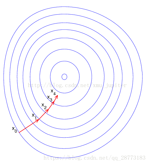
梯度算法就是以最快的速度进行最值的寻找,还记得高中时候求函数最值的方法吗,求其偏导数,令偏导数为0,批量梯度下降也是这个原理,但我们这里不做具体介绍.梯度上升算法最大的缺点就是只能找到局部最小值,因为从不同的初值进行梯度上升或下降的时候,其结果是不同的,如下图所示:
这里写图片描述
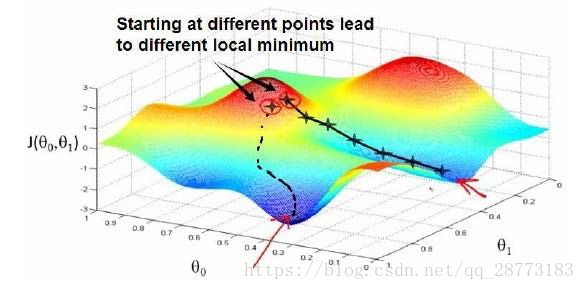
解决这个问题就可以参照贪心算法,我们在代码中用的也是随机梯度上升算法,代码如下:

#随机梯度上升算法
def stocGradAscent1(dataMatrix,classLabels,numIter=150):
    m,n = shape(dataMatrix)
    params =[]
    weights = ones(n)
    params.append(weights)
    for j in range(numIter):
        dataIndex = range(m)
        for i in range(m):
            alpha = 4/(1.0+j+i)+0.01
            randIndex = int(random.uniform(0,len(dataIndex))) #随机的选取起点
            h = sigmod(sum(dataMatrix[randIndex]*weights))
            error = classLabels[randIndex] - h
            weights = weights + alpha*error*dataMatrix[randIndex]
            del(dataIndex[randIndex])
        params.append(weights)
    return weights,params

在学习的过程中,最重要的就是代码中更新参数的那句代码如何推导:

weights = weights + alpha*error*dataMatrix[randIndex]

首先参数更新的方法是:

θ_{j} := θ_{j} - α \frac{\partial}{\partial θ_{j}} J (θ)

$\theta_j:=\theta_j-\alpha\frac{\partial}{\partial\theta_j}J(\theta)$
这里的重点是求偏导部分:

\begin{aligned} (63) & \frac{\partial}{\partial θ} J (θ) & = (1 - y) \frac{h_{θ}^{2} (x) e^{- θ^{T} X}}{1 - h_{θ} (x)} X - y \frac{h_{θ}^{2} (x) e^{- θ^{T} X}}{h_{θ} (x)} X \\ (64) & = e^{- θ^{T} X} X \frac{h_{θ} (x) (h_{θ} (x) - y)}{1 - h_{θ} (x)} \\ (65) & = X (h_{θ} (x) - y) \end{aligned}

$\begin{align} \frac{\partial}{\partial\theta}J(\theta)&=(1-y)\frac{h_{\theta}^{2}(x)e^{-\theta^{T}X}}{1-h_{\theta}(x)}X-y\frac{h_{\theta}^{2}(x)e^{-\theta^{T}X}}{h_{\theta}(x)}X \\ & = e^{-\theta^{T}X}X\frac{h_{\theta}(x)(h_{\theta}(x)-y)}{1-h_{\theta}(x)} \\ & =X(h_{\theta}(x)-y) \end{align}$

拟合结果和参数分析

对于testSet.txt的回归分类,我们画出决策边界,代码如下:

#!/usr/bin/env python
# -*- coding: utf-8 -*-
# @Time    :  //
# @Author  : FC
# @Site    : [email protected]
# @license : BSD

from numpy import *
from matplotlib import pyplot as plt

# 文件读取,并将data和label分开
# OUTPUT:dataMat:训练集;lableMat:训练集对应的标签
# Note:这里默认X0为1.0
def loadDataSet():
    dataMat = [];labelMat = []
    fr = open('testSet.txt')
    for line in fr.readlines():
        lineArr = line.strip().split()
        dataMat.append([1.0,float(lineArr[0]),float(lineArr[1])])
        labelMat.append(int(lineArr[2]))
    return array(dataMat),array(labelMat)
#sigmod函数
def sigmod(inX):
    return 1.0/(1+exp(-inX))

#梯度上升算法
def gradAscent(dataMatIn,classLabels):
    dataMatrix = mat(dataMatIn)
    labelMat = mat(classLabels).transpose()
    m,n = shape(dataMatrix)

    alpha = 0.001
    maxCycles = 500
    weights = ones((n,1))
    for k in range(maxCycles):
        h = sigmod(dataMatrix*weights)
        error = (labelMat - h)
        weights += alpha*dataMatrix.transpose()*error
    return weights

#数据划分图形化
def plotBestFit(wei):
    # weights = wei.getA() #将mat类型的wei转成array
    dataMat ,labelMat = loadDataSet()
    dataArr = array(dataMat)
    n = shape(dataArr)[0]
    xcord1 = [];ycord1 = []
    xcord2 = [];ycord2 = []
    for i in range(n):
        if int(labelMat[i]) == 1:
            xcord1.append(dataArr[i,1]);ycord1.append(dataArr[i,2])
        else:
            xcord2.append(dataArr[i,1]);ycord2.append(dataArr[i,2])
    fig = plt.figure()
    ax = fig.add_subplot(111)
    ax.scatter(xcord1,ycord1,s=30,c='red',marker='s')
    ax.scatter(xcord2,ycord2,s=30,c='green')
    x = arange(-3.0,3.0,0.1)
    y = (-weights[0]-weights[1]*x)/weights[2] #Z=w0X0+w1X1+w2X2,令Z=0,得到X1=-(w0X0+w1X1)/w2 此处X0=1
    ax.plot(x,y)
    plt.xlabel('X1');plt.ylabel('X2')
    plt.show()

def stocGradAscent0(dataMatrix,calssLabels):
    m,n = shape(dataMatrix)
    alpha = 0.01
    weights = ones(n)
    for i in range(m):
        h = sigmod(sum(dataMatrix[i]*weights))
        error = calssLabels[i] - h
        weights = weights + alpha*error*dataMatrix[i]
    return  weights

#随机梯度上升算法
def stocGradAscent1(dataMatrix,classLabels,numIter=150):
    m,n = shape(dataMatrix)
    params =[]
    weights = ones(n)
    params.append(weights)
    for j in range(numIter):
        dataIndex = range(m)
        for i in range(m):
            alpha = 4/(1.0+j+i)+0.01
            randIndex = int(random.uniform(0,len(dataIndex))) #随机的选取起点
            h = sigmod(sum(dataMatrix[randIndex]*weights))
            error = classLabels[randIndex] - h
            weights = weights + alpha*error*dataMatrix[randIndex]
            del(dataIndex[randIndex])
        params.append(weights)
    return weights,params

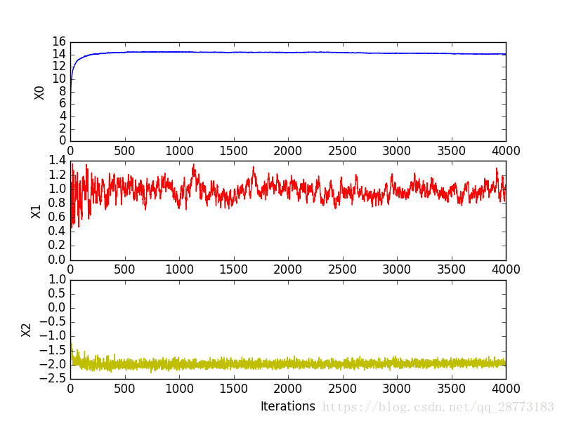
#迭代次数和回归系数的关系图
def PlotParams(numbers,params):
    fig = plt.figure()
    ax1 = fig.add_subplot(311)
    x1 = [];y1=[]
    for i in range(numbers):
        x1.append(i);y1.append(params[i][0])
    ax1.plot(x1,y1)
    plt.xlabel('Iterations')
    plt.ylabel('X0')

    ax2 = fig.add_subplot(312)
    x2 = [];y2=[]
    for i in range(numbers):
        x2.append(i);y2.append(params[i][1])
    ax2.plot(x2,y2,'r')
    plt.xlabel('Iterations')
    plt.ylabel('X1')

    ax1 = fig.add_subplot(313)
    x3 = [];y3=[]
    for i in range(numbers):
        x3.append(i);y3.append(params[i][2])
    ax1.plot(x3,y3,'y')
    plt.xlabel('Iterations')
    plt.ylabel('X2')
    plt.show()


if '__main__':
    dataMat,labelMat = loadDataSet()
    weights,params = stocGradAscent1(dataMat,labelMat,1000)
    plotBestFit(weights)

结果如下:
这里写图片描述

这里我们对学习速率进行了调整,学习速率在机器学习中也是很重要的,如果学习速率过大,很可能收敛不到最小值,学习速率过小,模型又会收敛得很慢,我们可以理解学习速率是步长,这就很好理解了,我们也可以可视化参数的变化,看出随机梯度算法不会出现参数的一直抖动,而且收敛较快.
! 这里写图片描述
最后是一个预测病马死亡率的例子,这里说一下如何处理缺失值:

1.使用可用特征的均值来填补缺失值
2.使用特殊值来填补缺失值,如-1
3.忽略有缺失值的样本
4.使用相似样本的均值添补缺失值
5.使用另外的机器学习算法预测缺失值

代码如下:

#!/usr/bin/env python
# -*- coding: utf-8 -*-
# @Time    :  //
# @Author  : FC
# @Site    : [email protected]
# @license : BSD
import  LogRegres
from numpy import *

def classifyVector(inX,weights):
    prob = LogRegres.sigmod(sum(inX*weights))
    if prob > 0.5 : return 1.0
    else: return 0.0


def colicTest():
    frTrain = open('horseColicTraining.txt')
    frTest = open('horseColicTest.txt')
    trainingSet = [];trainingLabels = []
    for line in frTrain.readlines():
        currLine = line.strip().split('\t')
        lineArr = []
        for i in range(len(currLine)-1):
            lineArr.append(float(currLine[i]))
        trainingSet.append(lineArr)
        trainingLabels.append(float(currLine[-1]))
    trainWeights,params = LogRegres.stocGradAscent1(array(trainingSet),trainingLabels,500)
    errorCount = 0;numTestVec = 0.0
    for line in frTest.readlines():
        numTestVec += 1.0
        currLine = line.strip().split('\t')
        lineArr = []
        for i in range(len(currLine)-1):
            lineArr.append(float(currLine[i]))

        if int(classifyVector(array(lineArr),trainWeights))!= int(currLine[-1]):
            errorCount += 1

    errorRate = errorCount/numTestVec
    print("the error rate of this is: %f" % errorRate)
    return errorRate

def multiTest():
    numTests = 10
    errorSum = 0
    for k in range(numTests):
        errorSum += colicTest()
    print("after %d iterations the average error rate is: %f" %(numTests,errorSum/numTests))

if '__main__':
    multiTest()

结果如下:

the error rate of this is: 0.358209
the error rate of this is: 0.343284
the error rate of this is: 0.417910
the error rate of this is: 0.313433
the error rate of this is: 0.343284
the error rate of this is: 0.358209
the error rate of this is: 0.343284
the error rate of this is: 0.388060
the error rate of this is: 0.328358
the error rate of this is: 0.343284
after 10 iterations the average error rate is: 0.353731

完整代码和数据集见我的Github:Logistic Regression