机器学习实战：基于Scikit-Learn和TensorFlow—第五章笔记

机器学习实战：基于Scikit-Learn和TensorFlow—第五章笔记

支持向量机

支持向量机（简称SVM）是一个功能强大并且全面的机器学习模型，它能够执行线性或非线性分类、回归，甚至是异常值检测任务。

线性SVM分类

选取鸢尾花数据集作为实验数据

from sklearn import datasets


iris = datasets.load_iris()
X = iris["data"][:, (2, 3)]  # petal length, petal width
y = iris["target"]

setosa_or_versicolor = (y == 0) | (y == 1)
X = X[setosa_or_versicolor]
# print(X)
# print("")
y = y[setosa_or_versicolor]
# print(y)

大间隔分类

SVM的基本思想可以用一些图来说明,如下实现：

import matplotlib.pyplot as plt
import numpy as np
from Chapter_5.demo.iris_data import X, y
from Chapter_5.demo.train_SVC import svm_clf


def plot_svc_decision_boundary(svm_clf, xmin, xmax):
    w = svm_clf.coef_[0]
    b = svm_clf.intercept_[0]
    # At the decision boundary, w0*x0 + w1*x1 + b = 0
    # => x1 = -w0/w1 * x0 - b/w1
    x0 = np.linspace(xmin, xmax, 200)
    decision_boundary = -w[0] / w[1] * x0 - b / w[1]
    margin = 1 / w[1]
    gutter_up = decision_boundary + margin
    gutter_down = decision_boundary - margin
    svs = svm_clf.support_vectors_
    plt.scatter(svs[:, 0], svs[:, 1], s=180, facecolors='#FFAAAA')
    plt.plot(x0, decision_boundary, "k-", linewidth=2)
    plt.plot(x0, gutter_up, "k--", linewidth=2)
    plt.plot(x0, gutter_down, "k--", linewidth=2)


# Bad models
x0 = np.linspace(0, 5.5, 200)
# print(x0)
pred_1 = 5 * x0 - 20
pred_2 = x0 - 1.8
pred_3 = 0.1 * x0 + 0.5
plt.figure(figsize=(12, 2.7))
plt.subplot(121)
plt.plot(x0, pred_1, "g--", linewidth=2)
plt.plot(x0, pred_2, "m-", linewidth=2)
plt.plot(x0, pred_3, "r-", linewidth=2)
plt.plot(X[:, 0][y == 1], X[:, 1][y == 1], "bs", label="Iris-Versicolor")
plt.plot(X[:, 0][y == 0], X[:, 1][y == 0], "yo", label="Iris-Setosa")
plt.xlabel("Petal length", fontsize=14)
plt.ylabel("Petal width", fontsize=14)
plt.legend(loc="upper left", fontsize=14)
plt.axis([0, 5.5, 0, 2])
plt.subplot(122)
plot_svc_decision_boundary(svm_clf, 0, 5.5)
plt.plot(X[:, 0][y == 1], X[:, 1][y == 1], "bs")
plt.plot(X[:, 0][y == 0], X[:, 1][y == 0], "yo")
plt.xlabel("Petal length", fontsize=14)
plt.axis([0, 5.5, 0, 2])
plt.show()

上面左图显示了三种可能的线性分类器的决策边界。其中虚线所代表的模型表现非常糟糕，甚至都无法正确实现分类。其余两个模型在这个训练集上表现堪称完美，但是它们的决策边界与实例过于接近，导致在面对新实例时，表现可能不会太好。

相比之下，右图中的实线代表SVM分类器的决策边界，这条线不仅分离了两个类别，并且尽可能远离了最近的训练实例。你可以将SVM分类器视为在类别之间拟合可能的最宽的街道（平行的虚线所示）。因此这也叫作大间隔分类（large margin classification）。

请注意，在街道以外的地方增加更多训练实例，不会对决策边界产生影响：也就是说它完全由位于街道边缘的实例所决定（或者称之为“支持”）。这些实例被称为支持向量（在上图已圈出）

对特征缩放的敏感度

SVM对特征的缩放非常敏感：

import matplotlib.pyplot as plt
import numpy as np
from sklearn.preprocessing import StandardScaler
from sklearn.svm import SVC
from Chapter_5.demo.plot_decision_boundary import plot_svc_decision_boundary

Xs = np.array([[1, 50], [5, 20], [3, 80], [5, 60]]).astype(np.float64)
ys = np.array([0, 0, 1, 1])
svm_clf = SVC(kernel="linear", C=100)
svm_clf.fit(Xs, ys)

plt.figure(figsize=(12, 3.2))
plt.subplot(121)
plt.plot(Xs[:, 0][ys == 1], Xs[:, 1][ys == 1], "bo")
plt.plot(Xs[:, 0][ys == 0], Xs[:, 1][ys == 0], "ms")
plot_svc_decision_boundary(svm_clf, 0, 6)
plt.xlabel("$x_0$", fontsize=20)
plt.ylabel("$x_1$  ", fontsize=20, rotation=0)
plt.title("Unscaled", fontsize=16)
plt.axis([0, 6, 0, 90])

scaler = StandardScaler()
X_scaled = scaler.fit_transform(Xs)
svm_clf.fit(X_scaled, ys)

plt.subplot(122)
plt.plot(X_scaled[:, 0][ys == 1], X_scaled[:, 1][ys == 1], "bo")
plt.plot(X_scaled[:, 0][ys == 0], X_scaled[:, 1][ys == 0], "ms")
plot_svc_decision_boundary(svm_clf, -2, 2)
plt.xlabel("$x_0$", fontsize=20)
plt.title("Scaled", fontsize=16)
plt.axis([-2, 2, -2, 2])
plt.show()

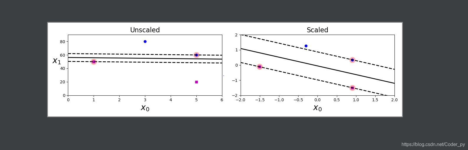
如上图所示，在左图中，垂直刻度比水平刻度大得多，因此可能的最宽的街道接近于水平。在特征缩放（例如使用Scikit-Learn的StandardScaler）后，决策边界看起来好很多（见上面右图）

软间隔分类

如果我们严格地让所有实例都不在街道上，并且位于正确的一边，这就是硬间隔分类。硬间隔分类有两个主要问题，首先，它只在数据是线性可分离的时候才有效；其次，它对异常值非常敏感。

扫描二维码关注公众号，回复： 8761942 查看本文章

硬间隔对异常值的敏感度：

import matplotlib.pyplot as plt
import numpy as np
from sklearn.preprocessing import StandardScaler
from sklearn.svm import SVC
from Chapter_5.demo.iris_data import X, y
from Chapter_5.demo.plot_decision_boundary import plot_svc_decision_boundary

X_outliers = np.array([[3.4, 1.3], [3.2, 0.8]])
y_outliers = np.array([0, 0])
Xo1 = np.concatenate([X, X_outliers[:1]], axis=0)
yo1 = np.concatenate([y, y_outliers[:1]], axis=0)
Xo2 = np.concatenate([X, X_outliers[1:]], axis=0)
yo2 = np.concatenate([y, y_outliers[1:]], axis=0)

svm_clf2 = SVC(kernel="linear", C=10**9)
svm_clf2.fit(Xo2, yo2)

plt.figure(figsize=(12,2.7))

plt.subplot(121)
plt.plot(Xo1[:, 0][yo1==1], Xo1[:, 1][yo1==1], "bs")
plt.plot(Xo1[:, 0][yo1==0], Xo1[:, 1][yo1==0], "yo")
plt.text(0.3, 1.0, "Impossible!", fontsize=24, color="red")
plt.xlabel("Petal length", fontsize=14)
plt.ylabel("Petal width", fontsize=14)
plt.annotate("Outlier",
             xy=(X_outliers[0][0], X_outliers[0][1]),
             xytext=(2.5, 1.7),
             ha="center",
             arrowprops=dict(facecolor='black', shrink=0.1),
             fontsize=16,
            )
plt.axis([0, 5.5, 0, 2])

plt.subplot(122)
plt.plot(Xo2[:, 0][yo2==1], Xo2[:, 1][yo2==1], "bs")
plt.plot(Xo2[:, 0][yo2==0], Xo2[:, 1][yo2==0], "yo")
plot_svc_decision_boundary(svm_clf2, 0, 5.5)
plt.xlabel("Petal length", fontsize=14)
plt.annotate("Outlier",
             xy=(X_outliers[1][0], X_outliers[1][1]),
             xytext=(3.2, 0.08),
             ha="center",
             arrowprops=dict(facecolor='black', shrink=0.1),
             fontsize=16,
            )
plt.axis([0, 5.5, 0, 2])
plt.show()

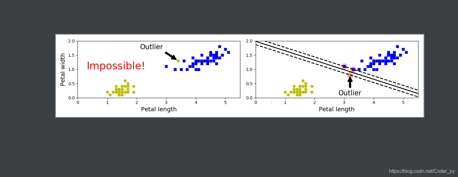
上图显示了有一个额外异常值的鸢尾花数据：左图的数据根本找不出硬间隔，而右图最终显示的决策边界与我们在前面中所看到的无异常值时的决策边界也大不相同，可能无法很好地泛化。

要避免这些问题，最好使用更灵活的模型。目标是尽可能在保持街道宽阔和限制间隔违例（即位于街道之上，甚至在错误的一边的实例）之间找到良好的平衡，这就是软间隔分类。

在Scikit-Learn的SVM类中，可以通过超参数C来控制这个平衡：C值越小，则街道越宽，但是间隔违例也会越多：

import numpy as np
from sklearn import datasets
from sklearn.pipeline import Pipeline
from sklearn.preprocessing import StandardScaler
from sklearn.svm import LinearSVC
import matplotlib.pyplot as plt
from Chapter_5.demo.plot_decision_boundary import plot_svc_decision_boundary

iris = datasets.load_iris()
X = iris["data"][:, (2, 3)]  # petal length, petal width
y = (iris["target"] == 2).astype(np.float64)  # Iris-Virginica

scaler = StandardScaler()
svm_clf1 = LinearSVC(C=1, loss="hinge", random_state=42)
svm_clf2 = LinearSVC(C=100, loss="hinge", random_state=42)

scaled_svm_clf1 = Pipeline([
    ("scaler", scaler),
    ("linear_svc", svm_clf1),
])
scaled_svm_clf2 = Pipeline([
    ("scaler", scaler),
    ("linear_svc", svm_clf2),
])
scaled_svm_clf1.fit(X, y)
scaled_svm_clf2.fit(X, y)

# Convert to unscaled parameters
b1 = svm_clf1.decision_function([-scaler.mean_ / scaler.scale_])
b2 = svm_clf2.decision_function([-scaler.mean_ / scaler.scale_])
w1 = svm_clf1.coef_[0] / scaler.scale_
w2 = svm_clf2.coef_[0] / scaler.scale_
svm_clf1.intercept_ = np.array([b1])
svm_clf2.intercept_ = np.array([b2])
svm_clf1.coef_ = np.array([w1])
svm_clf2.coef_ = np.array([w2])

# Find support vectors (LinearSVC does not do this automatically)
t = y * 2 - 1
support_vectors_idx1 = (t * (X.dot(w1) + b1) < 1).ravel()
support_vectors_idx2 = (t * (X.dot(w2) + b2) < 1).ravel()
svm_clf1.support_vectors_ = X[support_vectors_idx1]
svm_clf2.support_vectors_ = X[support_vectors_idx2]

scaled_svm_clf1.fit(X, y)
scaled_svm_clf2.fit(X, y)
plt.figure(figsize=(12, 3.2))
plt.subplot(121)
plt.plot(X[:, 0][y == 1], X[:, 1][y == 1], "g^", label="Iris-Virginica")
plt.plot(X[:, 0][y == 0], X[:, 1][y == 0], "bs", label="Iris-Versicolor")
plot_svc_decision_boundary(svm_clf1, 4, 6)
plt.xlabel("Petal length", fontsize=14)
plt.ylabel("Petal width", fontsize=14)
plt.legend(loc="upper left", fontsize=14)
plt.title("$C = {}$".format(svm_clf1.C), fontsize=16)
plt.axis([4, 6, 0.8, 2.8])

plt.subplot(122)
plt.plot(X[:, 0][y == 1], X[:, 1][y == 1], "g^")
plt.plot(X[:, 0][y == 0], X[:, 1][y == 0], "bs")
plot_svc_decision_boundary(svm_clf2, 4, 6)
plt.xlabel("Petal length", fontsize=14)
plt.title("$C = {}$".format(svm_clf2.C), fontsize=16)
plt.axis([4, 6, 0.8, 2.8])
plt.show()

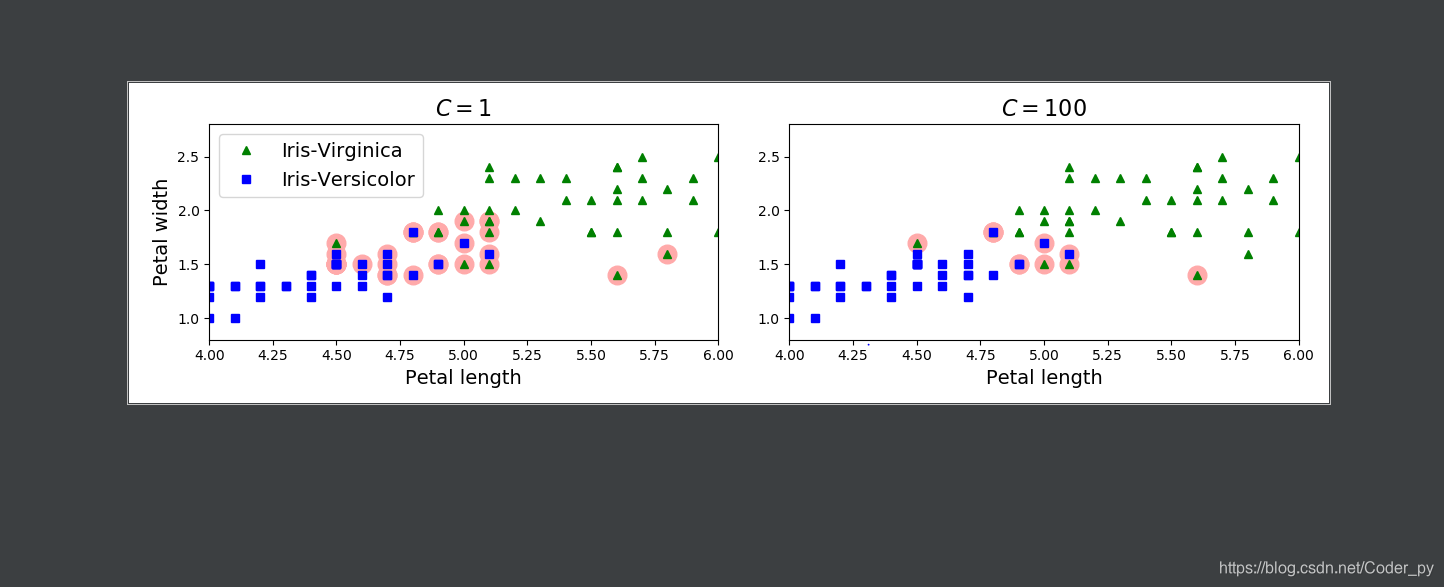
上图显示了在一个非线性可分离数据集上，两个软间隔SVM分类器各自的决策边界和间隔。左边使用了高C值，分类器的间隔违例较少，但是间隔也较小。右边使用了低C值，间隔大了很多，但是位于街道上的实例也更多。看起来第二个分类器的泛化效果更好，因为大多数间隔违例实际上都位于决策边界正确的一边，所以即便是在该训练集上，它做出的错误预测也会更少。

如果你的SVM模型过度拟合，可以试试通过降低C来进行正则化。

非线性SVM分类

虽然在许多情况下，线性SVM分类器是有效的，并且通常出人意料的好，但是，有很多数据集远不是线性可分离的。

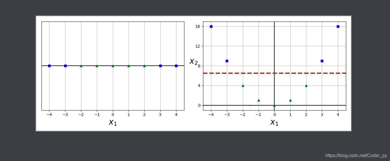
处理非线性数据集的方法之一是添加更多特征

多项式特征

某些情况下，这可能导致数据集变得线性可分离。参见图5-5的左图：这是一个简单的数据集，只有一个特征 $x_1$ ，可以看出，数据集线性不可分。但是如果添加第二个特征 $x_2$= $(x_1)^2$，生成的2D数据集则完全线性可分离:

import numpy as np
import matplotlib.pyplot as plt

X1D = np.linspace(-4, 4, 9).reshape(-1, 1)
X2D = np.c_[X1D, X1D**2]
y = np.array([0, 0, 1, 1, 1, 1, 1, 0, 0])

plt.figure(figsize=(11, 4))

plt.subplot(121)
plt.grid(True, which='both')
plt.axhline(y=0, color='k')
plt.plot(X1D[:, 0][y==0], np.zeros(4), "bs")
plt.plot(X1D[:, 0][y==1], np.zeros(5), "g^")
plt.gca().get_yaxis().set_ticks([])
plt.xlabel(r"$x_1$", fontsize=20)
plt.axis([-4.5, 4.5, -0.2, 0.2])

plt.subplot(122)
plt.grid(True, which='both')
plt.axhline(y=0, color='k')
plt.axvline(x=0, color='k')
plt.plot(X2D[:, 0][y==0], X2D[:, 1][y==0], "bs")
plt.plot(X2D[:, 0][y==1], X2D[:, 1][y==1], "g^")
plt.xlabel(r"$x_1$", fontsize=20)
plt.ylabel(r"$x_2$", fontsize=20, rotation=0)
plt.gca().get_yaxis().set_ticks([0, 4, 8, 12, 16])
plt.plot([-4.5, 4.5], [6.5, 6.5], "r--", linewidth=3)
plt.axis([-4.5, 4.5, -1, 17])
plt.subplots_adjust(right=1)
plt.show()

使用Scikit-Learn

用卫星数据集来进行实验：

from sklearn.datasets import make_moons
import matplotlib.pyplot as plt

X, y = make_moons(n_samples=100, noise=0.15, random_state=42)


def plot_dataset(X, y, axes):
    plt.plot(X[:, 0][y == 0], X[:, 1][y == 0], "bs")
    plt.plot(X[:, 0][y == 1], X[:, 1][y == 1], "g^")
    plt.axis(axes)
    plt.grid(True, which='both')
    plt.xlabel(r"$x_1$", fontsize=20)
    plt.ylabel(r"$x_2$", fontsize=20, rotation=0)


plot_dataset(X, y, [-1.5, 2.5, -1, 1.5])
plt.show()

搭建一条流水线：一个PolynomialFeatures转换器，接着一个StandardScaler，然后是LinearSVC:

from sklearn.datasets import make_moons
from sklearn.pipeline import Pipeline
from sklearn.preprocessing import PolynomialFeatures, StandardScaler
from sklearn.svm import LinearSVC
import matplotlib.pyplot as plt
import numpy as np

from Chapter_5.demo.make_moons import X, y, plot_dataset

polynomial_svm_clf = Pipeline([
    ("poly_features", PolynomialFeatures(degree=3)),
    ("scaler", StandardScaler()),
    ("svm_clf", LinearSVC(C=10, loss="hinge", random_state=42))
])

polynomial_svm_clf.fit(X, y)


def plot_predictions(clf, axes):
    x0s = np.linspace(axes[0], axes[1], 100)
    x1s = np.linspace(axes[2], axes[3], 100)
    x0, x1 = np.meshgrid(x0s, x1s)
    X = np.c_[x0.ravel(), x1.ravel()]
    y_pred = clf.predict(X).reshape(x0.shape)
    y_decision = clf.decision_function(X).reshape(x0.shape)
    plt.contourf(x0, x1, y_pred, cmap=plt.cm.brg, alpha=0.2)
    plt.contourf(x0, x1, y_decision, cmap=plt.cm.brg, alpha=0.1)


plot_predictions(polynomial_svm_clf, [-1.5, 2.5, -1, 1.5])
plot_dataset(X, y, [-1.5, 2.5, -1, 1.5])
plt.show()

多项式核

添加多项式特征实现起来非常简单，并且对所有的机器学习算法（不只是SVM）都非常有效。但问题是，如果多项式太低阶，处理不了非常复杂的数据集，而高阶则会创造出大量的特征，导致模型变得太慢。

幸运的是，使用SVM时，有一个魔术般的数学技巧可以应用，这就是核技巧.

它产生的结果就跟添加了许多多项式特征，甚至是非常高阶的多项式特征一样，但实际上并不需要真的添加。因为实际没有添加任何特征，所以也就不存在数量爆炸的组合特征了。这个技巧由SVC类来实现，我们看看在卫星数据集上的测试：

from sklearn.pipeline import Pipeline
from sklearn.preprocessing import StandardScaler
from sklearn.svm import SVC
import matplotlib.pyplot as plt
from Chapter_5.demo.Linear_SVM_classifier_using_polynomial_features import plot_predictions
from Chapter_5.demo.make_moons import X, y, plot_dataset

poly_kernel_svm_clf = Pipeline([
        ("scaler", StandardScaler()),
        ("svm_clf", SVC(kernel="poly", degree=3, coef0=1, C=5))
    ])
poly_kernel_svm_clf.fit(X, y)

poly100_kernel_svm_clf = Pipeline([
        ("scaler", StandardScaler()),
        ("svm_clf", SVC(kernel="poly", degree=10, coef0=100, C=5))
    ])
poly100_kernel_svm_clf.fit(X, y)

plt.figure(figsize=(11, 4))

plt.subplot(121)
plot_predictions(poly_kernel_svm_clf, [-1.5, 2.5, -1, 1.5])
plot_dataset(X, y, [-1.5, 2.5, -1, 1.5])
plt.title(r"$d=3, r=1, C=5$", fontsize=18)

plt.subplot(122)
plot_predictions(poly100_kernel_svm_clf, [-1.5, 2.5, -1, 1.5])
plot_dataset(X, y, [-1.5, 2.5, -1, 1.5])
plt.title(r"$d=10, r=100, C=5$", fontsize=18)
plt.show()

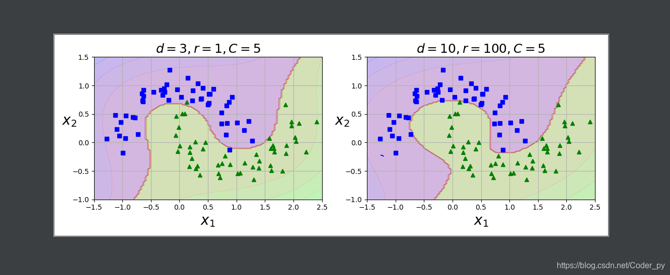
实验代码使用了一个3阶多项式内核训练SVM分类器。如上图的左图所示。而右图是另一个使用了10阶多项式核的SVM分类器。显然，如果模型过度拟合，你应该降低多项式阶数；反过来，如果拟合不足，则可以尝试使之提升。超参数coef0控制的是模型受高阶多项式还是低阶多项式影响的程度。

添加相似特征

解决非线性问题的另一种技术是添加相似特征。这些特征经过相似函数计算得出，相似函数可以测量每个实例与一个特定地标（landmark）之间的相似度。

使用高斯RBF的相似特征

import matplotlib.pyplot as plt
import numpy as np


def gaussian_rbf(x, landmark, gamma):
    return np.exp(-gamma * np.linalg.norm(x - landmark, axis=1) ** 2)


gamma = 0.3

X1D = np.linspace(-4, 4, 9).reshape(-1, 1)
X2D = np.c_[X1D, X1D ** 2]
x1s = np.linspace(-4.5, 4.5, 200).reshape(-1, 1)
x2s = gaussian_rbf(x1s, -2, gamma)
x3s = gaussian_rbf(x1s, 1, gamma)

XK = np.c_[gaussian_rbf(X1D, -2, gamma), gaussian_rbf(X1D, 1, gamma)]
yk = np.array([0, 0, 1, 1, 1, 1, 1, 0, 0])

plt.figure(figsize=(11, 4))

plt.subplot(121)
plt.grid(True, which='both')
plt.axhline(y=0, color='k')
plt.scatter(x=[-2, 1], y=[0, 0], s=150, alpha=0.5, c="red")
plt.plot(X1D[:, 0][yk == 0], np.zeros(4), "bs")
plt.plot(X1D[:, 0][yk == 1], np.zeros(5), "g^")
plt.plot(x1s, x2s, "g--")
plt.plot(x1s, x3s, "b:")
plt.gca().get_yaxis().set_ticks([0, 0.25, 0.5, 0.75, 1])
plt.xlabel(r"$x_1$", fontsize=20)
plt.ylabel(r"Similarity", fontsize=14)
plt.annotate(r'$\mathbf{x}$',
             xy=(X1D[3, 0], 0),
             xytext=(-0.5, 0.20),
             ha="center",
             arrowprops=dict(facecolor='black', shrink=0.1),
             fontsize=18,
             )
plt.text(-2, 0.9, "$x_2$", ha="center", fontsize=20)
plt.text(1, 0.9, "$x_3$", ha="center", fontsize=20)
plt.axis([-4.5, 4.5, -0.1, 1.1])

plt.subplot(122)
plt.grid(True, which='both')
plt.axhline(y=0, color='k')
plt.axvline(x=0, color='k')
plt.plot(XK[:, 0][yk == 0], XK[:, 1][yk == 0], "bs")
plt.plot(XK[:, 0][yk == 1], XK[:, 1][yk == 1], "g^")
plt.xlabel(r"$x_2$", fontsize=20)
plt.ylabel(r"$x_3$  ", fontsize=20, rotation=0)
plt.annotate(r'$\phi\left(\mathbf{x}\right)$',
             xy=(XK[3, 0], XK[3, 1]),
             xytext=(0.65, 0.50),
             ha="center",
             arrowprops=dict(facecolor='black', shrink=0.1),
             fontsize=18,
             )
plt.plot([-0.1, 1.1], [0.57, -0.1], "r--", linewidth=3)
plt.axis([-0.1, 1.1, -0.1, 1.1])
plt.subplots_adjust(right=1)
plt.show()

高斯RBF核函数

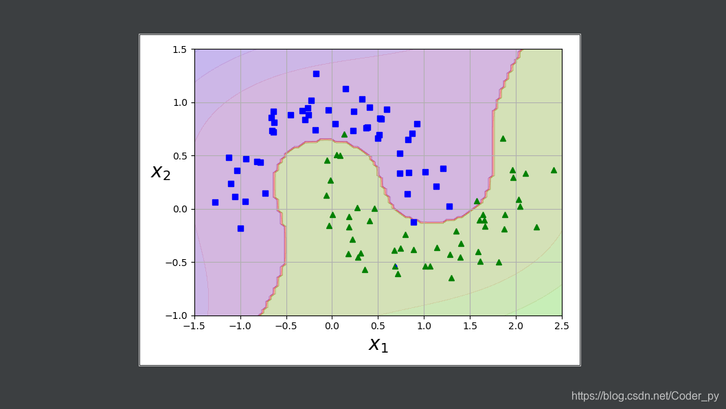
与多项式特征方法一样，相似特征法也可以用任意机器学习算法，但是要计算出所有附加特征，其计算代价可能非常昂贵，尤其是对大型训练集来说。然而，核技巧再一次施展了它的SVM魔术：它能够产生的结果就跟添加了许多相似特征一样，但实际上也并不需要添加。我们来使用SVC类试试高斯RBF核：

from sklearn.pipeline import Pipeline
from sklearn.preprocessing import StandardScaler
from sklearn.svm import SVC
import matplotlib.pyplot as plt

from Chapter_5.demo.Linear_SVM_classifier_using_polynomial_features import plot_predictions
from Chapter_5.demo.make_moons import plot_dataset, X, y

rbf_kernel_svm_clf = Pipeline([
        ("scaler", StandardScaler()),
        ("svm_clf", SVC(kernel="rbf", gamma=5, C=0.001))
    ])
rbf_kernel_svm_clf.fit(X, y)
from sklearn.svm import SVC

gamma1, gamma2 = 0.1, 5
C1, C2 = 0.001, 1000
hyperparams = (gamma1, C1), (gamma1, C2), (gamma2, C1), (gamma2, C2)

svm_clfs = []
for gamma, C in hyperparams:
    rbf_kernel_svm_clf = Pipeline([
            ("scaler", StandardScaler()),
            ("svm_clf", SVC(kernel="rbf", gamma=gamma, C=C))
        ])
    rbf_kernel_svm_clf.fit(X, y)
    svm_clfs.append(rbf_kernel_svm_clf)

plt.figure(figsize=(11, 7))

for i, svm_clf in enumerate(svm_clfs):
    plt.subplot(221 + i)
    plot_predictions(svm_clf, [-1.5, 2.5, -1, 1.5])
    plot_dataset(X, y, [-1.5, 2.5, -1, 1.5])
    gamma, C = hyperparams[i]
    plt.title(r"$\gamma = {}, C = {}$".format(gamma, C), fontsize=16)
plt.show()

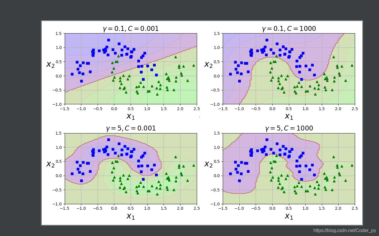
上图的左下方显示了这个模型。其他图显示了超参数gamma（）和C使用不同值时的模型。增加gamma值会使钟形曲线变得更窄（上图的左图），因此每个实例的影响范围随之变小：决策边界变得更不规则，开始围着单个实例绕弯。反过来，减小gamma值使钟形曲线变得更宽，因而每个实例的影响范围增大，决策边界变得更平坦。所以就像是一个正则化的超参数：模型过度拟合，就降低它的值，如果拟合不足则提升它的值（类似超参数C）。

SVM回归

SVM算法非常全面：它不仅支持线性和非线性分类，而且还支持线性和非线性回归。诀窍在于将目标反转一下：不再是尝试拟合两个类别之间可能的最宽的街道的同时限制间隔违例，SVM回归要做的是让尽可能多的实例位于街道上，同时限制间隔违例（也就是不在街道上的实例）。街道的宽度由超参数ε控制。

例子：

from sklearn.svm import LinearSVR
import numpy as np
import matplotlib.pyplot as plt

np.random.seed(42)
m = 50
X = 2 * np.random.rand(m, 1)
y = (4 + 3 * X + np.random.randn(m, 1)).ravel()

svm_reg = LinearSVR(epsilon=1.5, random_state=42)
svm_reg.fit(X, y)

svm_reg1 = LinearSVR(epsilon=1.5, random_state=42)
svm_reg2 = LinearSVR(epsilon=0.5, random_state=42)
svm_reg1.fit(X, y)
svm_reg2.fit(X, y)


def find_support_vectors(svm_reg, X, y):
    y_pred = svm_reg.predict(X)
    off_margin = (np.abs(y - y_pred) >= svm_reg.epsilon)
    return np.argwhere(off_margin)


svm_reg1.support_ = find_support_vectors(svm_reg1, X, y)
svm_reg2.support_ = find_support_vectors(svm_reg2, X, y)

eps_x1 = 1
eps_y_pred = svm_reg1.predict([[eps_x1]])


def plot_svm_regression(svm_reg, X, y, axes):
    x1s = np.linspace(axes[0], axes[1], 100).reshape(100, 1)
    y_pred = svm_reg.predict(x1s)
    plt.plot(x1s, y_pred, "k-", linewidth=2, label=r"$\hat{y}$")
    plt.plot(x1s, y_pred + svm_reg.epsilon, "k--")
    plt.plot(x1s, y_pred - svm_reg.epsilon, "k--")
    plt.scatter(X[svm_reg.support_], y[svm_reg.support_], s=180, facecolors='#FFAAAA')
    plt.plot(X, y, "bo")
    plt.xlabel(r"$x_1$", fontsize=18)
    plt.legend(loc="upper left", fontsize=18)
    plt.axis(axes)


plt.figure(figsize=(9, 4))
plt.subplot(121)
plot_svm_regression(svm_reg1, X, y, [0, 2, 3, 11])
plt.title(r"$\epsilon = {}$".format(svm_reg1.epsilon), fontsize=18)
plt.ylabel(r"$y$", fontsize=18, rotation=0)
# plt.plot([eps_x1, eps_x1], [eps_y_pred, eps_y_pred - svm_reg1.epsilon], "k-", linewidth=2)
plt.annotate(
    '', xy=(eps_x1, eps_y_pred), xycoords='data',
    xytext=(eps_x1, eps_y_pred - svm_reg1.epsilon),
    textcoords='data', arrowprops={'arrowstyle': '<->', 'linewidth': 1.5}
)
plt.text(0.91, 5.6, r"$\epsilon$", fontsize=20)
plt.subplot(122)
plot_svm_regression(svm_reg2, X, y, [0, 2, 3, 11])
plt.title(r"$\epsilon = {}$".format(svm_reg2.epsilon), fontsize=18)
plt.show()

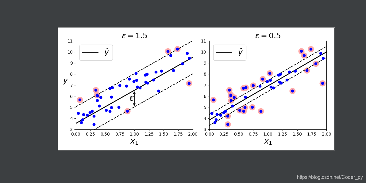
上图显示了用随机线性数据训练的两个线性SVM回归模型，一个间隔较大（ε＝1.5），另一个间隔较小（ε＝0.5）

在间隔内添加更多的实例不会影响模型的预测，所以这个模型被称为ε不敏感。

使用Scikit-Learn的LinearSVR

可以使用Scikit-Learn的LinearSVR类来执行线性SVM回归（训练数据需要先缩放并集中）

from sklearn.svm import SVR
import numpy as np
import matplotlib.pyplot as plt
from Chapter_5.demo.SVM_Regression import plot_svm_regression

m = 100
X = 2 * np.random.rand(m, 1) - 1
y = (0.2 + 0.1 * X + 0.5 * X**2 + np.random.randn(m, 1)/10).ravel()


svm_poly_reg1 = SVR(kernel="poly", degree=2, C=100, epsilon=0.1)
svm_poly_reg2 = SVR(kernel="poly", degree=2, C=0.01, epsilon=0.1)
svm_poly_reg1.fit(X, y)
svm_poly_reg2.fit(X, y)

plt.figure(figsize=(9, 4))
plt.subplot(121)
plot_svm_regression(svm_poly_reg1, X, y, [-1, 1, 0, 1])
plt.title(r"$degree={}, C={}, \epsilon = {}$".format(svm_poly_reg1.degree, svm_poly_reg1.C, svm_poly_reg1.epsilon), fontsize=18)
plt.ylabel(r"$y$", fontsize=18, rotation=0)
plt.subplot(122)
plot_svm_regression(svm_poly_reg2, X, y, [-1, 1, 0, 1])
plt.title(r"$degree={}, C={}, \epsilon = {}$".format(svm_poly_reg2.degree, svm_poly_reg2.C, svm_poly_reg2.epsilon), fontsize=18)
plt.show()

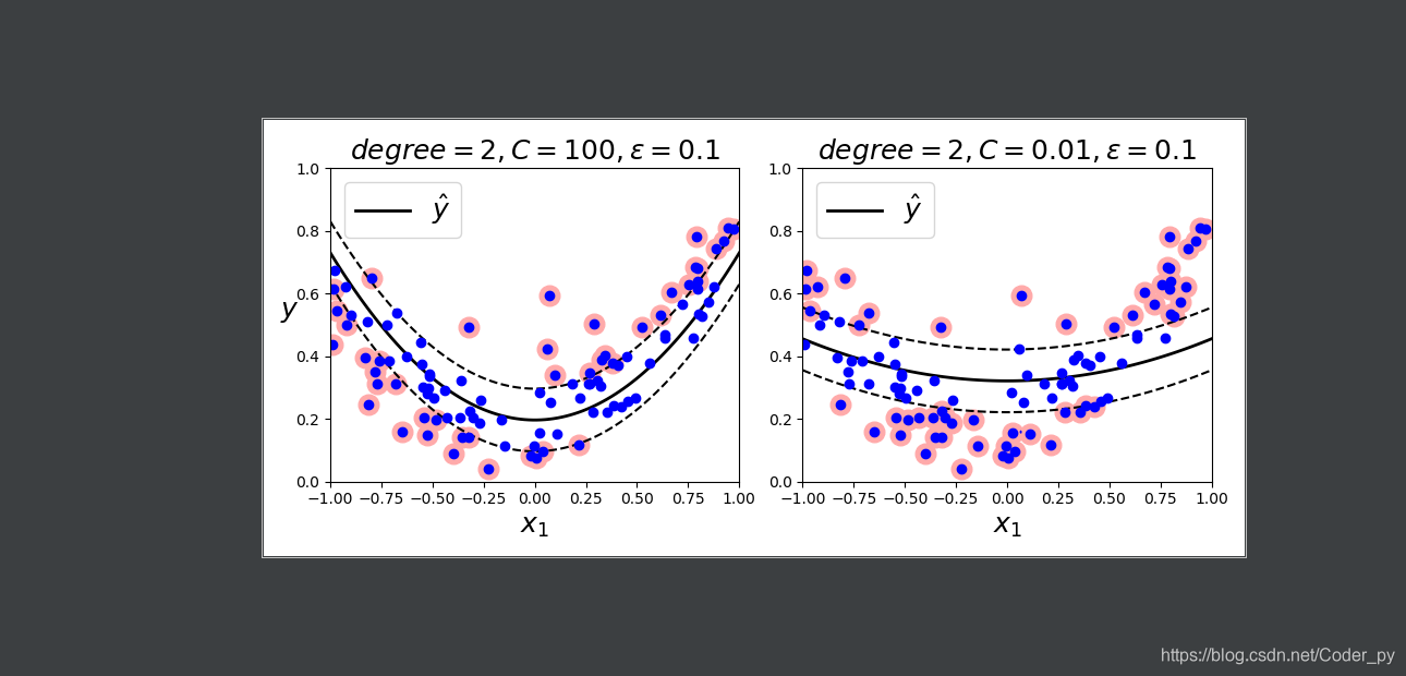
要解决非线性回归任务，可以使用核化的SVM模型。上图5-11显示了在一个随机二次训练集上，使用二阶多项式核的SVM回归。左图几乎没有正则化（C值很大），右图则过度正则化（C值很小）。