目录
论文阅读
代码解析
论文阅读
1.前言
自从AlexNet在2012年获得ImageNet冠军以来,卷积神经网络在计算机视觉中随处可见。为了获得更高的准确率,现在的趋势是让网络越来越深,越来越复杂。然而这些改进会影响到网络的大小和速度。在很多现实世界的应用中,比如机器人,自动驾驶,增强现实等,需要图像识别任务在有限的计算资源平台上做出及时的反应。
这篇论文描述了一个很高效的网络模型和两个超参数,来实现比较小的模型去满足手机和嵌入式设备的需求。
其实最近已经开始有一些论文对小而高效的论文感兴趣了。很多不同的尝试但是都可以总结为要么压缩预训练网络要么直接训练小型的网络。而这篇文章是要设计一种网络架构能够适应不同的资源限制。MobileNet主要关注的是优化延迟,而其他很多文章主要考虑网络大小而不考虑速度。
2.MobileNet结构
2.1 Depthwise Separable Convolution
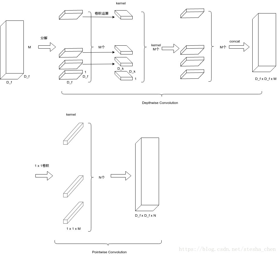
MobileNet的基础是Depthwise Separable Convolution(深度可分离卷积),这种卷积是将卷积进行了分解,分解成了一个depthwise convolution和一个1x1的卷积叫做pointwise convolution。Depthwise卷积是对input的每一个channel有一个filter,Pointwise卷积是对depthwise计算出来的结果进行1x1的卷积运算。标准的卷积运算是一步中就包含了filter计算和合并计算,然后直接将输入变成一个新的尺寸的输出。Depthwise separable convolution是将这个一步的操作分成了两层,一层做filter计算,一层做合并计算。这种分解的方式极大的减少了计算量和模型的大小。
先对上图的输入输出尺寸做一些说明。输入是尺寸为,输出的尺寸为
,
是输入的长宽,
是输入的channel(可以认为是depth),假设输出长宽不变
也是输出的长宽,
是输出的channel。
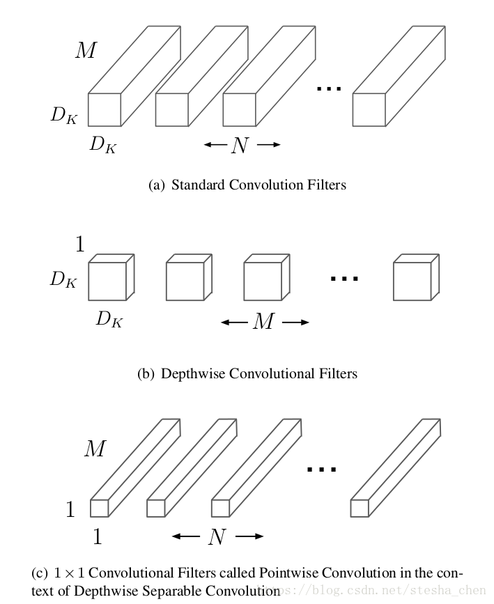
图(a)是标准的卷积运算需要的filter。对于标准的卷积计算方式,需要尺寸为的kernel,
是kernel的长宽。所以计算次数会是
图(b)是Depthwise卷积计算需要的filter。计算过程是将input的每一个channel都分开,为每一个channel设置一个kernel,因此需要个kernel,将每一个kernel和对应的channel进行卷积计算,可以得到
个结果,最后将这M个块合并得到
。计算次数是
图(c)是1x1的Pointwise卷积运算需要的filter。从图(b)得到的output作为这一步计算的输入,kernel为
,一共有
个kernel,进行卷积运算得到
。计算次数是
Depthwise和Pointwise的计算量加起来是完整的Depthwise Separable卷积运算的计算量。所以标准的卷积运算和Depthwise Separable卷积运算计算量的比例为:
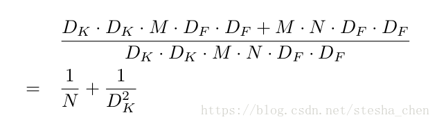
如果kernel的尺寸为3,那么使用Depthwise Separable卷积可以节省接近8/9的计算量。
2.2 网络结构
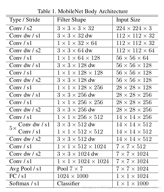
上图是作者提出的一种网络结构,除了最后一层,每一层后面都是跟着一个batchnorm和一个RELU激活函数。最后一层后面是跟着一个softmax用于分类。一共28层网络。下图就是原来的卷积计算和现在的depthwise卷积运算的对比。
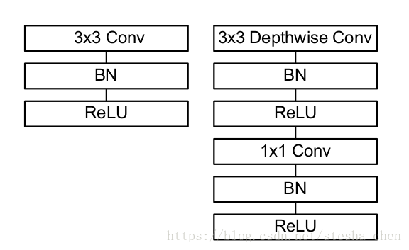
我们不仅仅需要减少运算次数,还需要保证这些计算能够很高效的执行。比如非结构化稀疏矩阵通常不会比密集矩阵计算速度快。我们的模型,几乎所有的计算都是在密集的1x1的卷积计算中,这可以用很高效的一般矩阵乘法(GEMM)来实现。常常卷积运算需要由im2col在存储中进行初步重新排序来映射到GEMM。但是1x1卷积不需要在存储中重新排序而可以直接有GEMM来实现,这是最优化的数值线性代数算法。
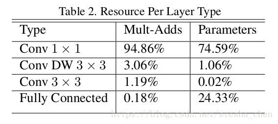
上图可以看出MobileNet有接近95%的计算都在1x1卷积上,也有接近75%的参数在1x1卷积上。
MobileNet用tensorflow实现,用的RMSProp非对称梯度下降。没有使用正则化和数据增强的技术,因为小的模型一般不会overfitting。另外需要使用很小的或者不使用weight decay。
2.3宽度因子(Width Multiplier):更薄的模型
如果需要模型更小更快,可以定义一个宽度因子,这个宽度因子可以让网络的每一层都变的更薄。如果input的channel是
就变为
,如果output channel是N就变为
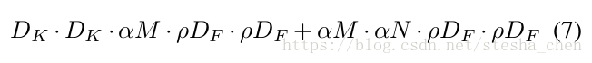
,那么在有宽度因子情况下的深度分离卷积运算的计算量公式就成了如下形式

,一般取值为1,0.75,0.5或者0.25。如果为1就是基本的mobilenet,如果小于1就是缩减了的mobilenet。宽度因子会缩小网络的计算量和参数,能够让原来的模型变成一个更小的模型,但是在精确度和模型尺寸之间需要权衡。而且如果修改了宽度因子,网络需要重头开始训练。
2.4分辨率因子(Resolution Multiplier):减少表达力
第二个减少计算量的超参数就是分辨率因子,这个因子是和input的长宽相乘,会缩小input的长宽而导致后面的每一层的长宽都缩小。
,一般让input的长宽为224,192,160和128。
代码解析
代码地址:mobilenet_v1
代码实现中关键的函数就两个,一个是mobilenet_v1_base,一个是mobilenet_v1,因为在mobilenet_v1中一开始就调用了mobilenet_v1_base,所以先从mobilenet_v1_base开始看。
1.mobilenet_v1_base
1.1 separable_conv2d
先了解一下代码中调用的slim.separable_conv2d函数,这是一个新的卷积运算的函数,这个函数的参数如下
separable_conv2d(
    inputs,
    num_outputs,
    kernel_size,
    depth_multiplier,
    stride=1,
    padding='SAME',
    data_format=DATA_FORMAT_NHWC,
    rate=1,
    activation_fn=tf.nn.relu,
    normalizer_fn=None,
    normalizer_params=None,
    weights_initializer=initializers.xavier_initializer(),
    pointwise_initializer=None,
    weights_regularizer=None,
    biases_initializer=tf.zeros_initializer(),
    biases_regularizer=None,
    reuse=None,
    variables_collections=None,
    outputs_collections=None,
    trainable=True,
    scope=None
)inputs: 是size为[batch_size, height, width, channels]的tensornum_outputs: 是pointwise卷积运算output的channel,如果为空,就不进行pointwise卷积运算。kernel_size: 是filter的size [kernel_height, kernel_width],如果filter的长宽一样可以只填入一个int值。depth_multiplier: 就是前面介绍过的宽度因子,在代码实现中改成了深度因子,因为是影响的channel,确实深度因子更合适。
这个函数可以直接实现Depthwise Separable Convolution的两个步骤,先进行depthwise卷积运算,再进行pointwise卷积运算。
1.2 循环
了解了这个新的卷积运算函数后再来看一下mobilenet_v1_base函数的实现。整个函数的主体是一个循环
for i, conv_def in enumerate(conv_defs):conv_defs是在代码的开头定义的_CONV_DEFS,当然我们也可以传入自己定义的结构。
_CONV_DEFS = [
    Conv(kernel=[3, 3], stride=2, depth=32),
    DepthSepConv(kernel=[3, 3], stride=1, depth=64),
    DepthSepConv(kernel=[3, 3], stride=2, depth=128),
    DepthSepConv(kernel=[3, 3], stride=1, depth=128),
    DepthSepConv(kernel=[3, 3], stride=2, depth=256),
    DepthSepConv(kernel=[3, 3], stride=1, depth=256),
    DepthSepConv(kernel=[3, 3], stride=2, depth=512),
    DepthSepConv(kernel=[3, 3], stride=1, depth=512),
    DepthSepConv(kernel=[3, 3], stride=1, depth=512),
    DepthSepConv(kernel=[3, 3], stride=1, depth=512),
    DepthSepConv(kernel=[3, 3], stride=1, depth=512),
    DepthSepConv(kernel=[3, 3], stride=1, depth=512),
    DepthSepConv(kernel=[3, 3], stride=2, depth=1024),
    DepthSepConv(kernel=[3, 3], stride=1, depth=1024)
]
在循环主体中,如果当前元素是Conv,就进行普通的卷积运算。
        if isinstance(conv_def, Conv):
          end_point = end_point_base
          if use_explicit_padding:
            net = _fixed_padding(net, conv_def.kernel)
          net = slim.conv2d(net, depth(conv_def.depth), conv_def.kernel,
                            stride=conv_def.stride,
                            normalizer_fn=slim.batch_norm,
                            scope=end_point)
          end_points[end_point] = net
          if end_point == final_endpoint:
            return net, end_points
如果当前元素是DepthSepConv,就进行separable_conv2d运算
        elif isinstance(conv_def, DepthSepConv):
          end_point = end_point_base + '_depthwise'

          # By passing filters=None
          # separable_conv2d produces only a depthwise convolution layer
          if use_explicit_padding:
            net = _fixed_padding(net, conv_def.kernel, layer_rate)
          net = slim.separable_conv2d(net, None, conv_def.kernel,
                                      depth_multiplier=1,
                                      stride=layer_stride,
                                      rate=layer_rate,
                                      normalizer_fn=slim.batch_norm,
                                      scope=end_point)
这样整个网络的主体就实现了。
2.mobilenet_v1
函数一开始就调用了mobilenet_v1_base,然后调用了avg_pool,最后就是softmax分类
      net, end_points = mobilenet_v1_base(inputs, scope=scope,
                                          min_depth=min_depth,
                                          depth_multiplier=depth_multiplier,
                                          conv_defs=conv_defs)
......
        net = slim.dropout(net, keep_prob=dropout_keep_prob, scope='Dropout_1b')
        logits = slim.conv2d(net, num_classes, [1, 1], activation_fn=None,
                             normalizer_fn=None, scope='Conv2d_1c_1x1')
......
      if prediction_fn:
        end_points['Predictions'] = prediction_fn(logits, scope='Predictions')
3.wrapped_partial
最后还需要说明一下wrapped_partial函数。
def wrapped_partial(func, *args, **kwargs):
  partial_func = functools.partial(func, *args, **kwargs)
  functools.update_wrapper(partial_func, func)
  return partial_func


mobilenet_v1_075 = wrapped_partial(mobilenet_v1, depth_multiplier=0.75)
mobilenet_v1_050 = wrapped_partial(mobilenet_v1, depth_multiplier=0.50)
mobilenet_v1_025 = wrapped_partial(mobilenet_v1, depth_multiplier=0.25)代码对为0.75,0.5和0.25进行了封装,这样当我们调用mobilenet_v1_075来构建网络的时候,depth_multiplier就已经设置为0.75了。
关于Resolution Multiplier的部分代码中并没有体现,因为他影响的是input的size,可以直接在传入input的时候进行处理。
以上为此篇的所有内容,感谢阅读,欢迎留言~