稀疏编码(Sparse Coding)是一种模拟哺乳动物视觉系统主视皮层V1区的视觉感知算法,NNSC(Non-Negative Sparse Coding,非负稀疏编码)是SC和非负矩阵分解相结合的一种编码算法。SparseAutoEncoder是深度学习的一种。需要利用SparseAutoEncoder训练出一个隐含层网络,对图像的特征进行学习。
特征的选取:
对57个训练样本的每一幅图片随机抽样1500个4×4个图像小块,4×4可显示一个眼的余角,4×4比8×8精确的多,使用NNSC训练,取256个特征,256个特征集合应该是一个超完备的特征集,关于特征数选择,我曾见过两种方式,一种是n*(n+2),n是块的大小,一种是spams的参考论文,10万个数据大约训练200个特征。
源码:
Bruno的sparsenet: http://redwood.berkeley.edu/bruno/sparsenet/
Andrew的Autoencoder: http://www.stanford.edu/class/cs294a/handouts.html
Exercise: http://deeplearning.stanford.edu/wiki/index.php/Exercise:Sparse_Autoencoder
参考代码:http://www.cnblogs.com/tornadomeet/archive/2013/03/20/2970724.html
http://ufldl.stanford.edu/wiki/index.php/UFLDL_Tutorial
参考资料: http://chentingpc.me/article/article.php?id=491 表情识别
http://max.book118.com/html/2014/0218/5979866.shtm 面向自然场景分类
代码和原理解析 http://blog.csdn.net/whiteinblue/article/details/20639629 *** 重要***
公式 http://wenku.baidu.com/link?url=YTAVWwO06J1aR0kil56oZfN5hjEo9_urlmazYUTufhd9O4MblGa5RhvIjgKjg2n1GgAT5nVWS1x26Lx449f6m0xtbYO0dkbmEbcNEPBrXSG
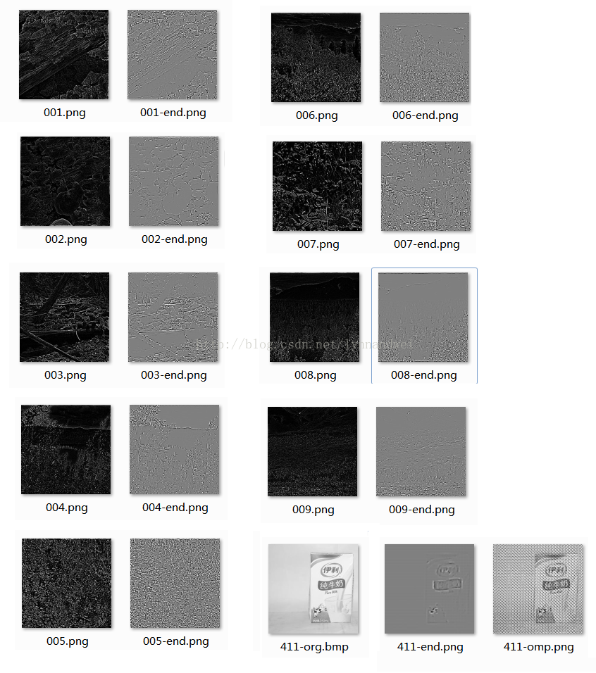
从两个方面来测试数据:一是用自带的十张图片,正在进行特征学习和提取。另外选择一些图片,进行dct变换后,去进行随机选取,用于特征学习。
1 将十张图随机选出10000个小特征,形成10000*64的矩阵,然后进行sparse coding 后,得到25*64的矩阵,形成特征的字典。(这一部分和网上大部分人展示的效果是基本一致的)
2 还原程序将原图通过字典还原,查看检查特征选取效果。但是 算法进行稀疏编码得到特征后,通过OMP算法还原这部分出错
整理了一下整个结构和思路。已经求出对应的参数。那么一张新的图,应该就能够直接用w1 w2来进行运算,得到结果。代码是一个64*10000的矩阵, 设置25*10000的隐层节点,目的就是求解 那个 64*25的字典。也就是W1的参数。 OMP部分是拿一张新的图像,在64*25的字典上 求一个线性分解。 但是 我困惑的是 W1这些参数也求出来了。 却还原不出正确的结果。看R的代码。他也是默认调用OMP的代码。公式在http://wenku.baidu.com/link?url=YTAVWwO06J1aR0kil56oZfN5hjEo9_urlmazYUTufhd9O4MblGa5RhvIjgKjg2n1GgAT5nVWS1x26Lx449f6m0xtbYO0dkbmEbcNEPBrXSG
3 优化是采用LBFGS 稀疏性惩罚 KL距离 http://www.cnblogs.com/tornadomeet/archive/2013/05/02/3053916.html http://hi.baidu.com/shdren09/item/e6441ec2bd495b0e0ad93aca
修改程序,从前9张图 获取到9999个块 提取之后 对 最后一张图用同样的参数,看输出结果和cost cost都在8左右。同一类应该是没有问题。
用其他的图片进行测试,效果一般,能看出图像,但是并不够好。
完成omp及相应算法 出来一个比较一般的结果 应该还是哪里有点什么问题。还没找到。 所以结果还有待优化。
修正参数。用牛奶的图片做测试。
%% CS294A/CS294W Programming Assignment Starter Code
% Instructions
% ------------
%
% This file contains code that helps you get started on the
% programming assignment. You will need to complete the code in sampleIMAGES.m,
% sparseAutoencoderCost.m and computeNumericalGradient.m.
% For the purpose of completing the assignment, you do not need to
% change the code in this file.
%
%%======================================================================
%% STEP 0: Here we provide the relevant parameters values that will
% allow your sparse autoencoder to get good filters; you do not need to
% change the parameters below.
visibleSize = 8*8; % number of input units
hiddenSize = 25; % number of hidden units
sparsityParam = 0.01; % desired average activation of the hidden units.
% (This was denoted by the Greek alphabet rho, which looks like a lower-case "p",
% in the lecture notes).
lambda = 0.0001; % weight decay parameter
beta = 3; % weight of sparsity penalty term
%%======================================================================
%% STEP 1: Implement sampleIMAGES
%
% After implementing sampleIMAGES, the display_network command should
% display a random sample of 200 patches from the dataset
patches = sampleIMAGES;
display_network(patches(:,randi(size(patches,2),200,1)),8);
% Obtain random parameters theta
theta = initializeParameters(hiddenSize, visibleSize);
%%======================================================================
%% STEP 2: Implement sparseAutoencoderCost
%
% You can implement all of the components (squared error cost, weight decay term,
% sparsity penalty) in the cost function at once, but it may be easier to do
% it step-by-step and run gradient checking (see STEP 3) after each step. We
% suggest implementing the sparseAutoencoderCost function using the following steps:
%
% (a) Implement forward propagation in your neural network, and implement the
% squared error term of the cost function. Implement backpropagation to
% compute the derivatives. Then (using lambda=beta=0), run Gradient Checking
% to verify that the calculations corresponding to the squared error cost
% term are correct.
%
% (b) Add in the weight decay term (in both the cost function and the derivative
% calculations), then re-run Gradient Checking to verify correctness.
%
% (c) Add in the sparsity penalty term, then re-run Gradient Checking to
% verify correctness.
%
% Feel free to change the training settings when debugging your
% code. (For example, reducing the training set size or
% number of hidden units may make your code run faster; and setting beta
% and/or lambda to zero may be helpful for debugging.) However, in your
% final submission of the visualized weights, please use parameters we
% gave in Step 0 above.
[cost, grad] = sparseAutoencoderCost(theta, visibleSize, hiddenSize, lambda, ...
sparsityParam, beta, patches);
grad
%%======================================================================
%% STEP 3: Gradient Checking
%
% Hint: If you are debugging your code, performing gradient checking on smaller models
% and smaller training sets (e.g., using only 10 training examples and 1-2 hidden
% units) may speed things up.
% First, lets make sure your numerical gradient computation is correct for a
% simple function. After you have implemented computeNumericalGradient.m,
% run the following:
%%%%
%checkNumericalGradient();
% Now we can use it to check your cost function and derivative calculations
% for the sparse autoencoder.
%%%%
%numgrad = computeNumericalGradient( @(x) sparseAutoencoderCost(x, visibleSize, ...
% hiddenSize, lambda, ...
% sparsityParam, beta, ...
% patches), theta);
% Use this to visually compare the gradients side by side
%%%%
%disp([numgrad grad]);
% Compare numerically computed gradients with the ones obtained from backpropagation
%%%%
%diff = norm(numgrad-grad)/norm(numgrad+grad);
%disp(diff); % Should be small. In our implementation, these values are
% usually less than 1e-9.
% When you got this working, Congratulations!!!
%%======================================================================
%% STEP 4: After verifying that your implementation of
% sparseAutoencoderCost is correct, You can start training your sparse
% autoencoder with minFunc (L-BFGS).
% Randomly initialize the parameters
theta = initializeParameters(hiddenSize, visibleSize);
% Use minFunc to minimize the function
addpath minFunc/
options.Method = 'lbfgs'; % Here, we use L-BFGS to optimize our cost
% function. Generally, for minFunc to work, you
% need a function pointer with two outputs: the
% function value and the gradient. In our problem,
% sparseAutoencoderCost.m satisfies this.
options.maxIter = 400; % Maximum number of iterations of L-BFGS to run
options.display = 'on';
[opttheta, cost] = minFunc( @(p) sparseAutoencoderCost(p, ...
visibleSize, hiddenSize, ...
lambda, sparsityParam, ...
beta, patches), ...
theta, options);
%%======================================================================
%% STEP 5: Visualization
W1 = reshape(opttheta(1:hiddenSize*visibleSize), hiddenSize, visibleSize);
display_network(W1', 12);
print -djpeg weights.jpg % save the visualization to a file
IMAGETEST = imread('D:\\Documents\\MATLAB\\test.jpg');
IMAGETESTGRAY = rgb2gray(IMAGETEST);
IMAGES_TEST = im2double(imresize(IMAGETESTGRAY,[256,256]));
imwrite(IMAGES_TEST ,['D:\\Documents\\MATLAB\\result\\411-org.bmp'])
%%STEP6 test the dictory is right
%%first cut the pic into small pieces.
%load IMAGES; % load images from disk
patchsize = 8; % we'll use 8x8 patches
% Initialize patches with zeros. Your code will fill in this matrix--one
% column per patch, 10000 columns.
% for i=1:10
%imshow(IMAGES(:,:,i));
% imwrite(IMAGES(:,:,i) ,['D:\\Documents\\MATLAB\\result\\',sprintf('%03d',i),'.png'])
[rowNum colNum] = size(IMAGES_TEST);
Image_T = zeros(rowNum,colNum);
Image_OMP = zeros(rowNum,colNum);
Image_OMP_test = zeros(rowNum,colNum);
Image_ORG = zeros(rowNum,colNum);
patches_result = zeros(patchsize*patchsize, rowNum*colNum/64);
patches_dict = zeros(patchsize*patchsize, rowNum*colNum/64);
for patchNum = 1:(colNum*rowNum/64)%
xPos =mod((patchNum-1)*8+1,colNum);
yPos = (floor((patchNum-1)*8/colNum))*8+1;
patches_result(:,patchNum) = reshape(IMAGES_TEST(xPos:xPos+7,yPos:yPos+7),64,1);
%%% patches = bsxfun(@minus, patches_result, mean(patches_result));
% Truncate to +/-3 standard deviations and scale to -1 to 1
%%%pstd = 3 * std(patches_result(:));
%%%patches_result = max(min(patches_result, pstd), -pstd) / pstd;
% Rescale from [-1,1] to [0.1,0.9]
%%%patches_result = (patches_result + 1) * 0.4 + 0.1;
Image_ORG(xPos:xPos+7,yPos:yPos+7)= reshape( patches_result(:,patchNum),patchsize,patchsize);
%%分配另外一个patches 然后存放比较后的字典,然后输出。
%% 从字典里比较最近的patches
% [rowW colW] = size(W1);
% FindResult= zeros(1,rowW);
% for k =1:rowW
% c=(patches_result(:,patchNum)'-W1(k,:)).^2;
% FindResult(k)= sqrt(sum(c(:)));
% FindResult(k)= pdist2(patches_result(:,patchNum)',W1(k,:));
%% T = bitxor(patches_result(:,patchNum)'*255, W1(k,:)*255)
%% FindResult(k)=length(find(A(T)~=0))
% end
% [x,m]=min(FindResult);
% patches_dict(:,patchNum) = W1(m,:);
W1 = reshape(opttheta(1:hiddenSize*visibleSize), hiddenSize, visibleSize);
W2 = reshape(opttheta(hiddenSize*visibleSize+1:2*hiddenSize*visibleSize), visibleSize, hiddenSize);
b1 = opttheta(2*hiddenSize*visibleSize+1:2*hiddenSize*visibleSize+hiddenSize);
b2 = opttheta(2*hiddenSize*visibleSize+hiddenSize+1:end);
rz2 = W1*patches_result+repmat(b1,1,colNum*rowNum/64);%注意这里一定要将b1向量复制扩展成m列的矩阵
ra2 = 1 ./ (1 + exp(-rz2));
rz3 = W2*ra2+repmat(b2,1,colNum*rowNum/64);
ra3 = 1 ./ (1 + exp(-rz3));
%patches_result(:,patchNum)
%ra3(:,patchNum)
Image_T(xPos:xPos+7,yPos:yPos+7)= reshape( ra3(:,patchNum),patchsize,patchsize);
% Tmp= IMAGES(xPos:xPos+7,yPos:yPos+7,imageNum);
% Tmp
% imwrite(Tmp ,['D:\\Documents\\MATLAB\\cut-sample\\',sprintf('%03d',(imageNum-1)*1000+patchNum),'.png'])
% function [A]=OMP(D,X,L);
%=============================================
% Sparse coding of a group of signals based on a given
% dictionary and specified number of atoms to use.
% ||X-DA||
% input arguments:
% D - the dictionary (its columns MUST be normalized).
% X - the signals to represent
% L - the max. number of coefficients for each signal.
% output arguments:
% A - sparse coefficient matrix.
%=============================================
X=patches_result(:,patchNum);
D= W1';
[nn,P]=size(X);
[nn,K]=size(D);
L =16;
for k=1:1:P,
a=[];
x=X(:,k); %the kth signal sample
residual=x; %initial the residual vector
indx=zeros(L,1); %initial the index vector
%the jth iter
for j=1:1:L,
%compute the inner product
proj=D'*residual;
%find the max value and its index
[maxVal,pos]=max(abs(proj));
%store the index
pos=pos(1);
indx(j)=pos;
%solve the Least squares problem.
a=pinv(D(:,indx(1:j)))*x;
%compute the residual in the new dictionary
residual=x-D(:,indx(1:j))*a;
%the precision is fill our demand.
% if sum(residual.^2) < 1e-6
% break;
% end
end;
temp=zeros(K,1);
temp(indx(1:j))=a;
A(:,k)=sparse(temp);
end;
patches_omptest = (A(:,k)'*W1 -0.1)/0.4 -1;
Image_OMP_test(xPos:xPos+7,yPos:yPos+7)= reshape( patches_omptest ,patchsize,patchsize);
%%%%OMP
s =patches_result(:,patchNum);
T = W1';
N = hiddenSize;
Size=size(T); % 观测矩阵大小
M=64; % 测量
hat_y=zeros(1,N); % 待重构的谱域(变换域)向量
Aug_t=[]; % 增量矩阵(初始值为空矩阵)
r_n=s; % 残差值
diedai = M/4;
pos_array=zeros(1,diedai);
for times=1:diedai % 迭代次数(稀疏度是测量的1/4) M/4
for col=1:N % 恢复矩阵的所有列向量
product(col)=abs(T(:,col)'*r_n); % 恢复矩阵的列向量和残差的投影系数(内积值)
end
[val,pos]=max(product); % 最大投影系数对应的位置
Aug_t=[Aug_t,T(:,pos)]; % 矩阵扩充
T(:,pos)=zeros(M,1); % 选中的列置零(实质上应该去掉,为了简单我把它置零)
aug_y=(Aug_t'*Aug_t)^(-1)*Aug_t'*s; % 最小二乘,使残差最小
r_n=s-Aug_t*aug_y; % 残差
pos_array(times)=pos; % 纪录最大投影系数的位置
if (norm(r_n)<0.05) % 残差足够小
break;
end
end
[tmpx,tmpy]= size(pos_array);
% 重构的向量
aug_y_16 = zeros(1,diedai);
aug_y_16 = double(aug_y_16);
aug_y_16(1,1:tmpy)=aug_y';
hat_y(pos_array)=aug_y_16;
rec= hat_y;
Image_OMP(xPos:xPos+7,yPos:yPos+7)= reshape( rec*W1,patchsize,patchsize);
end
resultcost = (0.5/(colNum*rowNum/64))*sum(sum((ra3-patches_result).^2));
resultcost
resultompcost = (0.5/(colNum*rowNum/64))*sum(sum((Image_OMP-Image_ORG).^2));
resultompcost
resultompcosttst = (0.5/(colNum*rowNum/64))*sum(sum((Image_OMP_test-Image_ORG).^2));
resultompcosttst
imshow(Image_T);
imwrite(Image_T ,['D:\\Documents\\MATLAB\\result\\411-end.png'])
imwrite(Image_OMP ,['D:\\Documents\\MATLAB\\result\\411-omp.png'])
imwrite(Image_OMP_test ,['D:\\Documents\\MATLAB\\result\\411-test.png'])
%%display_network(patches_dict);
%end;
function [cost,grad] = sparseAutoencoderCost(theta, visibleSize, hiddenSize, ...
lambda, sparsityParam, beta, data)
% visibleSize: the number of input units (probably 64)
% hiddenSize: the number of hidden units (probably 25)
% lambda: weight decay parameter
% sparsityParam: The desired average activation for the hidden units (denoted in the lecture
% notes by the greek alphabet rho, which looks like a lower-case "p").
% beta: weight of sparsity penalty term
% data: Our 64x10000 matrix containing the training data. So, data(:,i) is the i-th training example.
% The input theta is a vector (because minFunc expects the parameters to be a vector).
% We first convert theta to the (W1, W2, b1, b2) matrix/vector format, so that this
% follows the notation convention of the lecture notes.
W1 = reshape(theta(1:hiddenSize*visibleSize), hiddenSize, visibleSize);
W2 = reshape(theta(hiddenSize*visibleSize+1:2*hiddenSize*visibleSize), visibleSize, hiddenSize);
b1 = theta(2*hiddenSize*visibleSize+1:2*hiddenSize*visibleSize+hiddenSize);
b2 = theta(2*hiddenSize*visibleSize+hiddenSize+1:end);
% Cost and gradient variables (your code needs to compute these values).
% Here, we initialize them to zeros.
cost = 0;
W1grad = zeros(size(W1));
W2grad = zeros(size(W2));
b1grad = zeros(size(b1));
b2grad = zeros(size(b2));
%% ---------- YOUR CODE HERE --------------------------------------
% Instructions: Compute the cost/optimization objective J_sparse(W,b) for the Sparse Autoencoder,
% and the corresponding gradients W1grad, W2grad, b1grad, b2grad.
%
% W1grad, W2grad, b1grad and b2grad should be computed using backpropagation.
% Note that W1grad has the same dimensions as W1, b1grad has the same dimensions
% as b1, etc. Your code should set W1grad to be the partial derivative of J_sparse(W,b) with
% respect to W1. I.e., W1grad(i,j) should be the partial derivative of J_sparse(W,b)
% with respect to the input parameter W1(i,j). Thus, W1grad should be equal to the term
% [(1/m) \Delta W^{(1)} + \lambda W^{(1)}] in the last block of pseudo-code in Section 2.2
% of the lecture notes (and similarly for W2grad, b1grad, b2grad).
%
% Stated differently, if we were using batch gradient descent to optimize the parameters,
% the gradient descent update to W1 would be W1 := W1 - alpha * W1grad, and similarly for W2, b1, b2.
%
% http://deeplearning.stanford.edu/wiki/index.php/Autoencoders_and_Sparsity
Jcost = 0;%直接误差
Jweight = 0;%权值惩罚
Jsparse = 0;%稀疏性惩罚
[n m] = size(data);%m为样本的个数,n为样本的特征数
%前向算法计算各神经网络节点的线性组合值和active值
z2 = W1*data+repmat(b1,1,m);%注意这里一定要将b1向量复制扩展成m列的矩阵
a2 = sigmoid(z2);
z3 = W2*a2+repmat(b2,1,m);
a3 = sigmoid(z3);
% 计算预测产生的误差
Jcost = (0.5/m)*sum(sum((a3-data).^2));
%计算权值惩罚项
Jweight = (1/2)*(sum(sum(W1.^2))+sum(sum(W2.^2)));
%计算稀释性规则项
rho = (1/m).*sum(a2,2);%求出第一个隐含层的平均值向量
Jsparse = sum(sparsityParam.*log(sparsityParam./rho)+ ...
(1-sparsityParam).*log((1-sparsityParam)./(1-rho)));
%损失函数的总表达式
cost = Jcost+lambda*Jweight+beta*Jsparse;
%反向算法求出每个节点的误差值
d3 = -(data-a3).*sigmoidInv(z3);
sterm = beta*(-sparsityParam./rho+(1-sparsityParam)./(1-rho));%因为加入了稀疏规则项,所以
%计算偏导时需要引入该项
d2 = (W2'*d3+repmat(sterm,1,m)).*sigmoidInv(z2);
%计算W1grad
W1grad = W1grad+d2*data';
W1grad = (1/m)*W1grad+lambda*W1;
%计算W2grad
W2grad = W2grad+d3*a2';
W2grad = (1/m).*W2grad+lambda*W2;
%计算b1grad
b1grad = b1grad+sum(d2,2);
b1grad = (1/m)*b1grad;%注意b的偏导是一个向量,所以这里应该把每一行的值累加起来
%计算b2grad
b2grad = b2grad+sum(d3,2);
b2grad = (1/m)*b2grad;
%-------------------------------------------------------------------
% After computing the cost and gradient, we will convert the gradients back
% to a vector format (suitable for minFunc). Specifically, we will unroll
% your gradient matrices into a vector.
grad = [W1grad(:) ; W2grad(:) ; b1grad(:) ; b2grad(:)];
end
%-------------------------------------------------------------------
% Here's an implementation of the sigmoid function, which you may find useful
% in your computation of the costs and the gradients. This inputs a (row or
% column) vector (say (z1, z2, z3)) and returns (f(z1), f(z2), f(z3)).
function sigm = sigmoid(x)
sigm = 1 ./ (1 + exp(-x));
end
function sigmInv = sigmoidInv(x)
sigmInv = sigmoid(x).*(1-sigmoid(x));
end
function patches = sampleIMAGES()
% sampleIMAGES
% Returns 10000 patches for training
%load IMAGES; % load images from disk
%for i=1:10
%imshow(IMAGES(:,:,i));
%IMAGES(:,:,i)
% end;
oldPwd = pwd;
imgDir='D:\\Documents\\MATLAB\\milk';
imgDir2='D:\\Documents\\MATLAB\\milk\\%s';
IMAGES = zeros(256,256,25)
cd(imgDir);
x = dir;
listOfImages = [];
for i = 1:length(x),
if x(i).isdir == 0,
listOfImages = [listOfImages; x(i)];
end;
end;
fid=imgDir2;
for j = 1:length(listOfImages)
fileName = listOfImages(j).name;
rfid=sprintf(fid,fileName);
Irgb=imread(rfid);
Igray = rgb2gray(Irgb);
IMAGES(:,:,j) =im2double( imresize(Igray,[256,256]));
IMAGES(:,:,j)
end
cd(oldPwd);
patchsize = 8; % we'll use 8x8 patches
numpatches = 10000;
% Initialize patches with zeros. Your code will fill in this matrix--one
% column per patch, 10000 columns.
patches = zeros(patchsize*patchsize, numpatches);
%% ---------- YOUR CODE HERE --------------------------------------
% Instructions: Fill in the variable called "patches" using data
% from IMAGES.
%
% IMAGES is a 3D array containing 10 images
% For instance, IMAGES(:,:,6) is a 512x512 array containing the 6th image,
% and you can type "imagesc(IMAGES(:,:,6)), colormap gray;" to visualize
% it. (The contrast on these images look a bit off because they have
% been preprocessed using using "whitening." See the lecture notes for
% more details.) As a second example, IMAGES(21:30,21:30,1) is an image
% patch corresponding to the pixels in the block (21,21) to (30,30) of
% Image 1
for imageNum = 1:25%在每张图片中随机选取1000个patch,共10000个patch
[rowNum colNum] = size(IMAGES(:,:,imageNum));
for patchNum = 1:400%实现每张图片选取1000个patch
xPos = randi([1,rowNum-patchsize+1]);
yPos = randi([1, colNum-patchsize+1]);
patches(:,(imageNum-1)*400+patchNum) = reshape(IMAGES(xPos:xPos+7,yPos:yPos+7,...
imageNum),64,1);
% Tmp= IMAGES(xPos:xPos+7,yPos:yPos+7,imageNum);
% Tmp
% imwrite(Tmp ,['D:\\Documents\\MATLAB\\cut-sample\\',sprintf('%03d',(imageNum-1)*1000+patchNum),'.png'])
end
end
%% ---------------------------------------------------------------
% For the autoencoder to work well we need to normalize the data
% Specifically, since the output of the network is bounded between [0,1]
% (due to the sigmoid activation function), we have to make sure
% the range of pixel values is also bounded between [0,1]
patches = normalizeData(patches);
end
%% ---------------------------------------------------------------
function patches = normalizeData(patches)
% Squash data to [0.1, 0.9] since we use sigmoid as the activation
% function in the output layer
% Remove DC (mean of images).
patches = bsxfun(@minus, patches, mean(patches));
% Truncate to +/-3 standard deviations and scale to -1 to 1
pstd = 3 * std(patches(:));
patches = max(min(patches, pstd), -pstd) / pstd;
% Rescale from [-1,1] to [0.1,0.9]
patches = (patches + 1) * 0.4 + 0.1;
end
function theta = initializeParameters(hiddenSize, visibleSize)
%% Initialize parameters randomly based on layer sizes.
r = sqrt(6) / sqrt(hiddenSize+visibleSize+1); % we'll choose weights uniformly from the interval [-r, r]
W1 = rand(hiddenSize, visibleSize) * 2 * r - r;
W2 = rand(visibleSize, hiddenSize) * 2 * r - r;
b1 = zeros(hiddenSize, 1);
b2 = zeros(visibleSize, 1);
% Convert weights and bias gradients to the vector form.
% This step will "unroll" (flatten and concatenate together) all
% your parameters into a vector, which can then be used with minFunc.
theta = [W1(:) ; W2(:) ; b1(:) ; b2(:)];
end
function numgrad = computeNumericalGradient(J, theta)
% numgrad = computeNumericalGradient(J, theta)
% theta: a vector of parameters
% J: a function that outputs a real-number. Calling y = J(theta) will return the
% function value at theta.
% Initialize numgrad with zeros
numgrad = zeros(size(theta));
%% ---------- YOUR CODE HERE --------------------------------------
% Instructions:
% Implement numerical gradient checking, and return the result in numgrad.
% (See Section 2.3 of the lecture notes.)
% You should write code so that numgrad(i) is (the numerical approximation to) the
% partial derivative of J with respect to the i-th input argument, evaluated at theta.
% I.e., numgrad(i) should be the (approximately) the partial derivative of J with
% respect to theta(i).
%
% Hint: You will probably want to compute the elements of numgrad one at a time.
epsilon = 1e-4;
n = size(theta,1);
E = eye(n);
for i = 1:n
delta = E(:,i)*epsilon;
numgrad(i) = (J(theta+delta)-J(theta-delta))/(epsilon*2.0);
end
%% ---------------------------------------------------------------
end