题目链接:点击打开链接
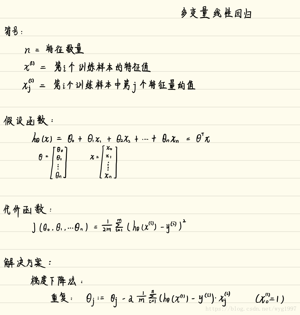
先附上笔记
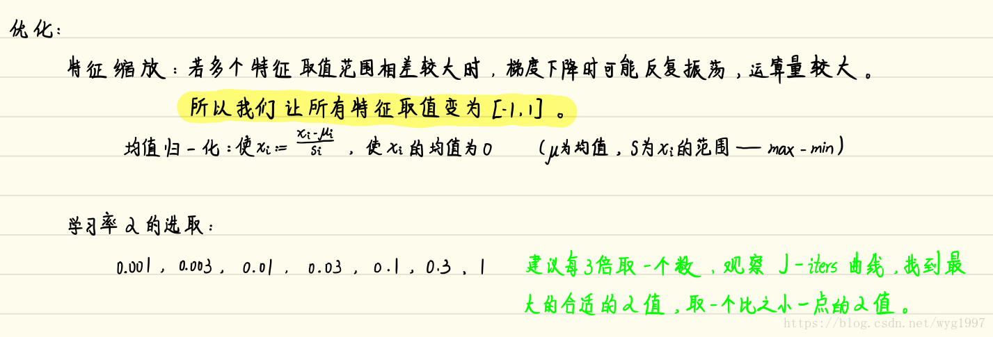
然后是程序的运行流程:
首先是对数据的特征缩放,使用均值归一化的方式:
featureNormalize.m
function [X_norm, mu, sigma] = featureNormalize(X)
%FEATURENORMALIZE Normalizes the features in X
%   FEATURENORMALIZE(X) returns a normalized version of X where
%   the mean value of each feature is 0 and the standard deviation
%   is 1. This is often a good preprocessing step to do when
%   working with learning algorithms.

% You need to set these values correctly
X_norm = X;
mu = zeros(1, size(X, 2));
sigma = zeros(1, size(X, 2));

% ====================== YOUR CODE HERE ======================
% Instructions: First, for each feature dimension, compute the mean
%               of the feature and subtract it from the dataset,
%               storing the mean value in mu. Next, compute the
%               standard deviation of each feature and divide
%               each feature by it's standard deviation, storing
%               the standard deviation in sigma.
%
%               Note that X is a matrix where each column is a
%               feature and each row is an example. You need
%               to perform the normalization separately for
%               each feature.
%
% Hint: You might find the 'mean' and 'std' functions useful.
%

mu = mean(X);
sigma = sum(X);
for i = 1:size(X,2)
   X_norm(:,i) = (X(:,i) - mu(1,i))/std(X(:,i));
end


% ============================================================

end
然后是计算代价函数(和单变量的差别不大)
computeCostMulti.m
function J = computeCostMulti(X, y, theta)
%COMPUTECOSTMULTI Compute cost for linear regression with multiple variables
%   J = COMPUTECOSTMULTI(X, y, theta) computes the cost of using theta as the
%   parameter for linear regression to fit the data points in X and y

% Initialize some useful values
m = length(y); % number of training examples

% You need to return the following variables correctly
J = 0;

% ====================== YOUR CODE HERE ======================
% Instructions: Compute the cost of a particular choice of theta
%               You should set J to the cost.

temp = X*theta-y;
J = temp'*temp/2.0/m;


% =========================================================================

end
使用梯度下降法求出θ
gradientDescentMulti.m
function [theta, J_history] = gradientDescentMulti(X, y, theta, alpha, num_iters)
%GRADIENTDESCENTMULTI Performs gradient descent to learn theta
%   theta = GRADIENTDESCENTMULTI(x, y, theta, alpha, num_iters) updates theta by
%   taking num_iters gradient steps with learning rate alpha

% Initialize some useful values
m = length(y); % number of training examples
J_history = zeros(num_iters, 1);

for iter = 1:num_iters

    % ====================== YOUR CODE HERE ======================
    % Instructions: Perform a single gradient step on the parameter vector
    %               theta.
    %
    % Hint: While debugging, it can be useful to print out the values
    %       of the cost function (computeCostMulti) and gradient here.
    %

    theta = theta - alpha/m*X'*(X*theta - y);


    % ============================================================

    % Save the cost J in every iteration
    J_history(iter) = computeCostMulti(X, y, theta);

end

end
这些效果图展示了α值和梯度下降速度的关系
(通过调整ex1_multi.m中的α值)
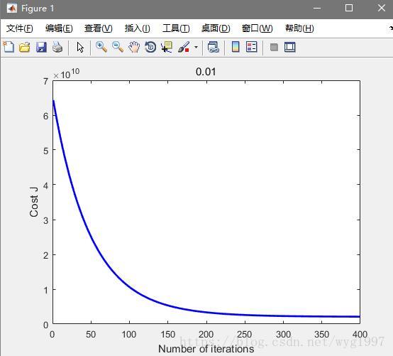
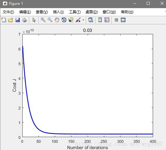
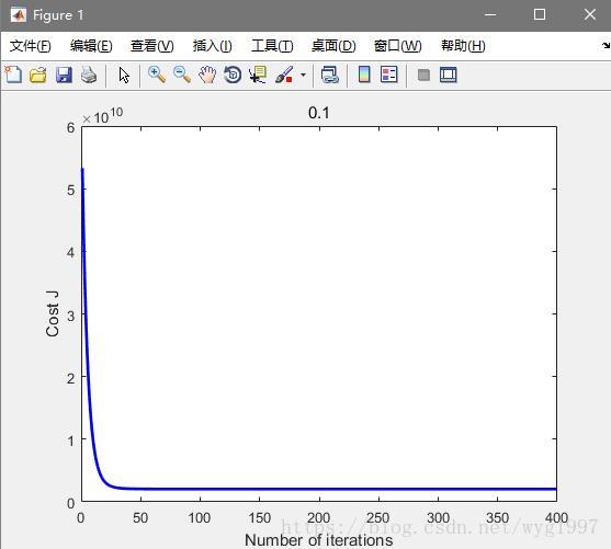
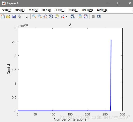
最后一个取3的时候J开始上升,所以α可以取1,可以更快的计算出结果