吴恩达机器学习课后作业_逻辑回归1_线性可分

逻辑回归1_线性可分问题

问题描述:根据学生的两门学生成绩，预测该学生是否会被大学录取

---

目录
1、加载数据集
2、可视化数据集
3、添加列
4、提取特征与标签
5、定义sigmoid函数
6、损失函数
7、梯度下降
8、预测
9、准确率
10、决策边界（补充知识点）

---

import numpy as np
import pandas as pd
import matplotlib.pyplot as plt

1、加载数据集

# 1、加载数据集
data = pd.read_csv('./ex2data1.txt', names=['score1','score2','possibility'])
data.head()

	score1	score2	possibility
0	34.623660	78.024693	0
1	30.286711	43.894998	0
2	35.847409	72.902198	0
3	60.182599	86.308552	1
4	79.032736	75.344376	1

2、可视化数据集

# 2、可视化数据集
fig, ax = plt.subplots()
ax.scatter(data[data['possibility']==0]['score1'], data[data['possibility']==0]['score2'],c='r', marker='x', label='y=0')
ax.scatter(data[data['possibility']==1]['score1'], data[data['possibility']==1]['score2'],c='b',marker='o', label='y=1')
ax.legend()
ax.set(xlabel='score1',
       ylabel='score2')
plt.show()

3、添加列

# 3、添加列
data.insert(0,'ones',1)
data.head()

	ones	score1	score2	possibility
0	1	34.623660	78.024693	0
1	1	30.286711	43.894998	0
2	1	35.847409	72.902198	0
3	1	60.182599	86.308552	1
4	1	79.032736	75.344376	1

4、提取特征与标签

# 4、提取特征与标签
X = data.iloc[:, 0:-1].values
y = data.iloc[:, -1].values.reshape(-1, 1)
print(X.shape)
print(y.shape)

(100, 3)
(100, 1)

5、定义sigmoid函数

# 5、定义sigmoid函数
def sigmoid(a):
    return 1 / (1 + np.exp(-a))  

6、损失函数

# 6、损失函数
def cost_function(X, y, theta):
    hx = sigmoid(X@theta)
    cost = -np.sum(y * np.log(hx) + (1 - y) * np.log(1- hx)) / len(X)
    return cost

# 初始化参数
theta = np.zeros((3,1))
cost_init = cost_function(X, y, theta)
cost_init

0.6931471805599453

7、梯度下降

# 7、梯度下降
def gradient_descent(X, y, theta, alpha, iters):
    costs =[]
    for i in range(iters):
        hx = sigmoid(X@theta)
        theta  = theta -(alpha / len(X))  * X.T @ (hx - y)
        cost = cost_function(X, y, theta)
        costs.append(cost)
        
        if i % 10000 == 0:
            print(cost)
    return theta,costs

iters = 200000
alpha = 0.004
theta_final,costs =  gradient_descent(X,y,theta,alpha,iters)

1.9886538578930084
2.7066763807478127
5.159653459570274
1.3288041261254437
1.6525865746034032
0.334478044895226
0.8401579263488419
0.9593734096464135
0.3227041012186722
0.46007956427143226
0.5862147537785243
0.5563008562186095
0.5181653708713927
0.47602965884191434
0.43309711107262444
0.39138015073568366
0.3524418831806119
0.31772301939998754
0.2883949718298337
0.26496140669529517

theta_final

array([[-23.77445621],
       [  0.20684474],
       [  0.19996049]])

8、预测

# 8、预测
def predict(X,theta):
    prob = sigmoid(X@theta)
    return [1 if x >= 0.5 else 0 for x in prob]

prob = sigmoid(X@theta)
y_pred = [1 if x >= 0.5 else 0 for x in prob]
len(y_pred)

100

y_ = np.array(predict(X,theta_final))  # 把列表转换成一维数组
y_.shape

(100,)

y_pre = y_.reshape(len(y_),1)  # 把一维数组 转换成 二维数组
y_pre.shape

(100, 1)

c = np.array([[1],[0]])
c

array([[1],
       [0]])

d = np.array([[1],[1]])
c==d

array([[ True],
       [False]])

acc_test  = np.mean(c == d)
acc_test

0.5

9、准确率

# 9、准确率
acc = np.mean(y_pred == y)
acc

0.6

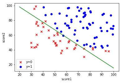
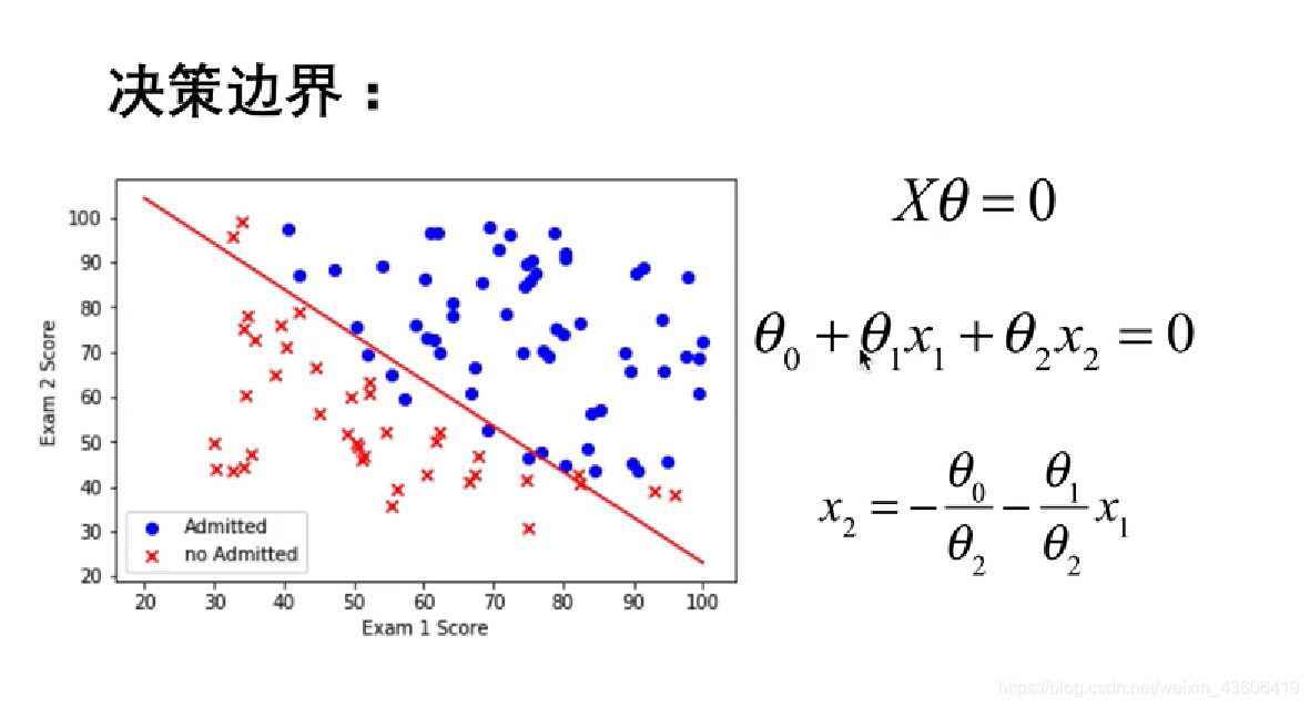
10、决策边界

补充知识点:
绘制的决策边界：
就是 hx = 0 的 那条直线，带入最后得到的最优参数。

# 10、决策边界
coef1 = - theta_final[0,0] / theta_final[2,0]
coef2 = - theta_final[1,0] / theta_final[2,0]

x = np.linspace(20,100,100)
f = coef1 + coef2 * x

fig,ax = plt.subplots()
ax.scatter(data[data['possibility']==0]['score1'],data[data['possibility']==0]['score2'],c='r',marker='x',label='y=0')
ax.scatter(data[data['possibility']==1]['score1'],data[data['possibility']==1]['score2'],c='b',marker='o',label='y=1')
ax.legend()
ax.set(xlabel='score1',
       ylabel='score2')

ax.plot(x,f,c='g')
plt.show()