文章目录
一、scara机器人运动学正解
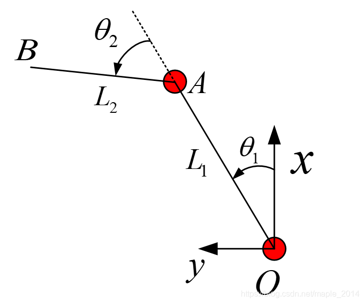
末端 B B B的 x x x坐标为向量 O A \bf{OA} OA与向量 A B \bf{AB} AB在 x x x轴上投影之和,末端 B B B的 y y y坐标亦然:
{ x = L 1 c o s θ 1 + L 2 c o s ( θ 1 + θ 2 ) y = L 1 s i n θ 1 + L 2 s i n ( θ 1 + θ 2 ) (1) \left \{ \begin{array}{c} x=L_1cos\theta_1+L_2cos(\theta_1+\theta_2) \\ \tag 1 y=L_1sin\theta_1+L_2sin(\theta_1+\theta_2) \end{array}\right. {
x=L1cosθ1+L2cos(θ1+θ2)y=L1sinθ1+L2sin(θ1+θ2)(1)
第三轴为丝杆上下平移运动,设丝杆螺距 s s s,末端 B B B的 z z z坐标:
z = θ 3 s 2 π (2) z=\frac{\theta_3s}{2\pi} \tag 2 z=2πθ3s(2)
末端 B B B的姿态角 c c c:
c = θ 1 + θ 2 + θ 4 (3) c=\theta_1+ \theta_2+ \theta_4 \tag 3 c=θ1+θ2+θ4(3)
综上,scara机器人的运动学正解为:
{ x = L 1 c o s θ 1 + L 2 c o s ( θ 1 + θ 2 ) y = L 1 s i n θ 1 + L 2 s i n ( θ 1 + θ 2 ) z = θ 3 s 2 π c = θ 1 + θ 2 + θ 4 (4) \begin{cases} x=L_1cos\theta_1+L_2cos(\theta_1+\theta_2) \\ y=L_1sin\theta_1+L_2sin(\theta_1+\theta_2) \\ z=\frac{\theta_3s}{2\pi} \\ c=\theta_1+ \theta_2+ \theta_4 \tag 4 \end{cases} ⎩⎪⎪⎪⎨⎪⎪⎪⎧x=L1cosθ1+L2cos(θ1+θ2)y=L1sinθ1+L2sin(θ1+θ2)z=2πθ3sc=θ1+θ2+θ4(4)
二、scara机器人运动学逆解
1、正装scara机器人运动学逆解
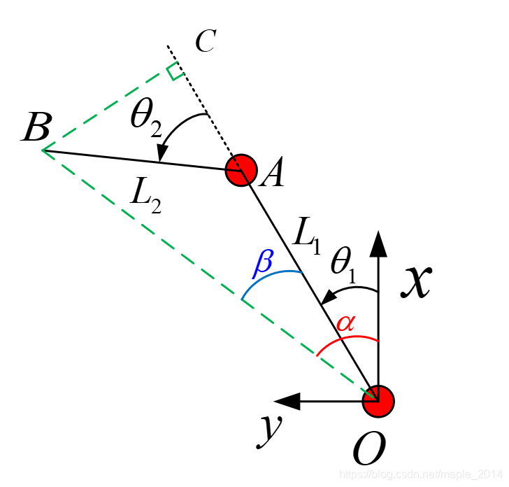
连接 O B OB OB,过 B B B作 B C BC BC垂直于 O A OA OA于 C C C,在 Δ O A B \Delta OAB ΔOAB中,由余弦定理:
c o s ( π − θ 2 ) = L 1 2 + L 2 2 − ( x 2 + y 2 ) 2 L 1 L 2 (5) cos(\pi-\theta_2)=\frac{L_1^2+L_2^2-(x^2+y^2)}{2L_1L_2}\tag 5 cos(π−θ2)=2L1L2L12+L22−(x2+y2)(5)
记 c 2 = c o s θ 2 c_2=cos\theta_2 c2=cosθ2,式(5)可写成:
c 2 = x 2 + y 2 − L 1 2 − L 2 2 2 L 1 L 2 (6) c_2=\frac{x^2+y^2-L_1^2-L_2^2}{2L_1L_2}\tag 6 c2=2L1L2x2+y2−L12−L22(6)
记 s 2 = s i n θ 2 s_2=sin\theta_2 s2=sinθ2,则 s 2 s_2 s2有两个解:
s 2 = ± 1 − c 2 2 (7) s_2=\pm\sqrt{1-c_2^2}\tag 7 s2=±1−c22(7)
取正数解,机器人处于右手系(right handcoor);取负数解,机器人处于左手系(left handcoor);特殊地,若 s 2 = 0 s_2=0 s2=0,机器人处于奇异位置(singular position),此时 θ 2 = k π ( k ∈ Z ) \theta_2=k\pi(k\in{Z}) θ2=kπ(k∈Z),一般 θ 2 ∈ { − 2 π , − π , 0 , π , 2 π } \theta_2\in{\{-2\pi,-\pi,0,\pi,2\pi}\} θ2∈{
−2π,−π,0,π,2π}。
至此,可求得 θ 2 \theta_2 θ2:
θ 2 = a t a n 2 ( s 2 , c 2 ) (8) \theta_2=atan2(s_2,c_2)\tag 8 θ2=atan2(s2,c2)(8)
如上图,易得:
α = a t a n 2 ( y , x ) (9) \alpha=atan2(y,x)\tag 9 α=atan2(y,x)(9)
在 Δ O B C \Delta OBC ΔOBC中,记 r = ∥ O B ∥ r=\|OB\| r=∥OB∥:
s i n β = ∥ B C ∥ ∥ O B ∥ = L 2 s 2 r (10) sin\beta=\frac{\|BC\|}{\|OB\|}=\frac{L_2s_2}{r}\tag {10} sinβ=∥OB∥∥BC∥=rL2s2(10)
c o s β = ∥ O C ∥ ∥ O B ∥ = ∥ O A ∥ + ∥ A C ∥ ∥ O B ∥ = L 1 + L 2 c 2 r (11) cos\beta=\frac{\|OC\|}{\|OB\|}=\frac{\|OA\|+\|AC\|}{\|OB\|}=\frac{L_1+L_2c_2}{r}\tag {11} cosβ=∥OB∥∥OC∥=∥OB∥∥OA∥+∥AC∥=rL1+L2c2(11)
由于 r > 0 r>0 r>0,由式 ( 10 ) (10) (10)和式 ( 11 ) (11) (11)得:
β = a t a n 2 ( L 2 s 2 , L 1 + L 2 c 2 ) (12) \beta=atan2(L_2s_2,L_1+L_2c_2)\tag {12} β=atan2(L2s2,L1+L2c2)(12)
至此,可求得 θ 1 \theta_1 θ1:
θ 1 = α − β = a t a n 2 ( y , x ) − a t a n 2 ( L 2 s 2 , L 1 + L 2 c 2 ) (13) \theta_1=\alpha-\beta=atan2(y,x)-atan2(L_2s_2,L_1+L_2c_2)\tag {13} θ1=α−β=atan2(y,x)−atan2(L2s2,L1+L2c2)(13)
由式 ( 4 ) (4) (4)容易求得 θ 3 \theta_3 θ3和 θ 4 \theta_4 θ4。
综上,正装scara机器人的运动学逆解为:
{ θ 1 = a t a n 2 ( y , x ) − a t a n 2 ( L 2 s 2 , L 1 + L 2 c 2 ) θ 2 = a t a n 2 ( s 2 , c 2 ) θ 3 = 2 π z s θ 4 = c − θ 1 − θ 2 (14) \begin{cases} \theta_1=atan2(y,x)-atan2(L_2s_2,L_1+L_2c_2) \\ \theta_2=atan2(s_2,c_2) \\ \theta_3=\frac{2\pi z}{s} \\ \theta_4=c-\theta_1-\theta_2 \tag {14} \end{cases} ⎩⎪⎪⎪⎨⎪⎪⎪⎧θ1=atan2(y,x)−atan2(L2s2,L1+L2c2)θ2=atan2(s2,c2)θ3=s2πzθ4=c−θ1−θ2(14)
在求解 θ 2 \theta_2 θ2时,完全可以根据式 ( 6 ) (6) (6)用反余弦函数 a c o s acos acos求得,但这里采用了双变量反正切函数 a t a n 2 atan2 atan2,至于原因,可以参见这篇博文:为什么机器人运动学逆解最好采用双变量反正切函数atan2而不用反正/余弦函数?
由于 a t a n 2 atan2 atan2的值域为 [ − π , π ] [-\pi,\pi] [−π,π],可得关节角度 θ 1 \theta_1 θ1在 − 2 π -2\pi −2π和 2 π 2\pi 2π之间(区间左端点 − 2 π -2\pi −2π和区间右端点 2 π 2\pi 2π不一定能达到), θ 2 ∈ [ − π , π ] \theta_2\in[-\pi,\pi] θ2∈[−π,π], θ 3 \theta_3 θ3范围与丝杆螺距 s s s和 z z z轴的行程有关, θ 4 \theta_4 θ4一般范围在 [ − 2 π , 2 π ] [-2\pi,2\pi] [−2π,2π]。对于正装scara机器人,为避免机构干涉,一般 θ 1 ∈ [ − 3 π 4 , 3 π 4 ] \theta_1\in[-\frac{3\pi}{4},\frac{3\pi}{4}] θ1∈[−43π,43π], θ 2 ∈ [ − 2 π 3 , 2 π 3 ] \theta_2\in[-\frac{2\pi}{3},\frac{2\pi}{3}] θ2∈[−32π,32π]。 式 ( 14 ) (14) (14)的运动学逆解无法做到使机器人在工作空间360°无死角运动,需要将其推广,使得 θ 1 ∈ [ − 2 π , 2 π ] \theta_1\in[-2\pi,2\pi] θ1∈[−2π,2π]且 θ 2 ∈ [ − 2 π , 2 π ] \theta_2\in[-2\pi,2\pi] θ2∈[−2π,2π],即吊装scara机器人关节1和关节2的角度范围。
2、吊装scara机器人运动学逆解
通过式 ( 14 ) (14) (14)计算得到 θ 1 \theta_1 θ1与 θ 2 \theta_2 θ2后,增加关节1与关节2角度标志位flagJ1与flagJ2,利用以下的规则,可以将 θ 1 \theta_1 θ1与 θ 2 \theta_2 θ2范围限定在 [ − 2 π , 2 π ] [-2\pi,2\pi] [−2π,2π],实现吊装scara机器人360°无死角运动。
将 θ 1 \theta_1 θ1范围变换到 [ − π , π ] [-\pi,\pi] [−π,π]:
若 θ 1 < − π \theta_1<-\pi θ1<−π,则 θ 1 = θ 1 + 2 π \theta_1=\theta_1+2\pi θ1=θ1+2π;
若 θ 1 > π \theta_1>\pi θ1>π,则 θ 1 = θ 1 − 2 π \theta_1=\theta_1-2\pi θ1=θ1−2π
对于 θ 1 \theta_1 θ1,当 f l a g J 1 = 1 flagJ1=1 flagJ1=1时:
若 θ 1 ≥ 0 \theta_1\geq0 θ1≥0,则 θ 1 = θ 1 − 2 π \theta_1=\theta_1-2\pi θ1=θ1−2π;
若 θ 1 < 0 \theta_1<0 θ1<0,则 θ 1 = θ 1 + 2 π \theta_1=\theta_1+2\pi θ1=θ1+2π
对于 θ 2 \theta_2 θ2,当 f l a g 2 = 1 flag2=1 flag2=1时:
若 θ 2 ≥ 0 \theta_2\geq0 θ2≥0,则 θ 2 = θ 2 − 2 π \theta_2=\theta_2-2\pi θ2=θ2−2π;
若 θ 2 < 0 \theta_2<0 θ2<0, θ 2 = θ 2 + 2 π \theta_2=\theta_2+2\pi θ2=θ2+2π
θ 4 = c − θ 1 − θ 2 \theta_4=c-\theta_1-\theta_2 θ4=c−θ1−θ2
3、几个值得思考的问题
(1)、手系handcoor的确定
当 θ 2 ∈ ( 0 , π ) ⋃ ( − 2 π , − π ) \theta_2\in(0,\pi) \bigcup(-2\pi,-\pi) θ2∈(0,π)⋃(−2π,−π)时,机器人处于右手系,此时 h a n d c o o r = 1 handcoor=1 handcoor=1
当 θ 2 ∈ ( − π , 0 ) ⋃ ( π , 2 π ) \theta_2\in(-\pi,0) \bigcup(\pi,2\pi) θ2∈(−π,0)⋃(π,2π)时,机器人处于左手系,此时 h a n d c o o r = 0 handcoor=0 handcoor=0
特别的,当 θ 2 ∈ { − 2 π , − π , 0 , π , 2 π } \theta_2\in{\{-2\pi,-\pi,0,\pi,2\pi}\} θ2∈{
−2π,−π,0,π,2π},机器人处于奇异位置。
当机器人示教了一个点位, θ 2 \theta_2 θ2便确定了,因此机器人当前示教点的手系便确定。
(2)、标志位flagJ1与flagJ2的确定
当 θ 1 ∈ [ − π , π ] \theta_1\in[-\pi,\pi] θ1∈[−π,π]时, f l a g J 1 = 0 flagJ1=0 flagJ1=0;否则, f l a g J 1 = 1 flagJ1=1 flagJ1=1。
当 θ 2 ∈ [ − π , π ] \theta_2\in[-\pi,\pi] θ2∈[−π,π]时, f l a g J 2 = 0 flagJ2=0 flagJ2=0;否则, f l a g J 2 = 1 flagJ2=1 flagJ2=1。
当手系handcoor确定后,便可以根据手系选逆解。当标志位flagJ1与flagJ2确定后,便可以确定关节角度值是否需要 ± 2 π \pm 2\pi ±2π。
(3)、选取最短关节路径逆解
在做笛卡尔空间插补(如直线、圆弧、样条插补等)时,如果 θ 1 ∈ [ − 2 π , 2 π ] \theta_1\in[-2\pi,2\pi] θ1∈[−2π,2π]且 θ 2 ∈ [ − 2 π , 2 π ] \theta_2\in[-2\pi,2\pi] θ2∈[−2π,2π],求逆解过程可能会有 ± 2 π \pm 2\pi ±2π的跳变。这时需要通过对比上一次关节位置,选取最短关节路径的解,以达到插补过程关节位置平滑变化,此时不再需要标志位flagJ1与flagJ2。
三、正逆解正确性验证
1、单点验证
(1)在 [ − 2 π , 2 π ] [-2\pi, 2\pi] [−2π,2π]中随机生成4个关节角度(模拟示教过程)
(2)计算标志位flagJ1和flagJ2,手系handcoor
(3)计算正运动学
(4)计算逆运动学
(5)逆运动学结果与随机生成的关节角度作差,验证运动学正逆解的正确性
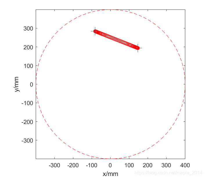
2、直线验证
(1)在 [ − 2 π , 2 π ] [-2\pi,2\pi] [−2π,2π]中随机生成4个关节角度,计算手系handcoor(模拟示教过程)
(2)运动学正解计算直线起点坐标(x,y,z,c)
(3)在工作空间里随机获取直线的终点x,y坐标,z在[-50mm,50mm]里随机生成,
c在[-30°, 30°]里随机生成,手系与起点的相同(模拟示教过程)
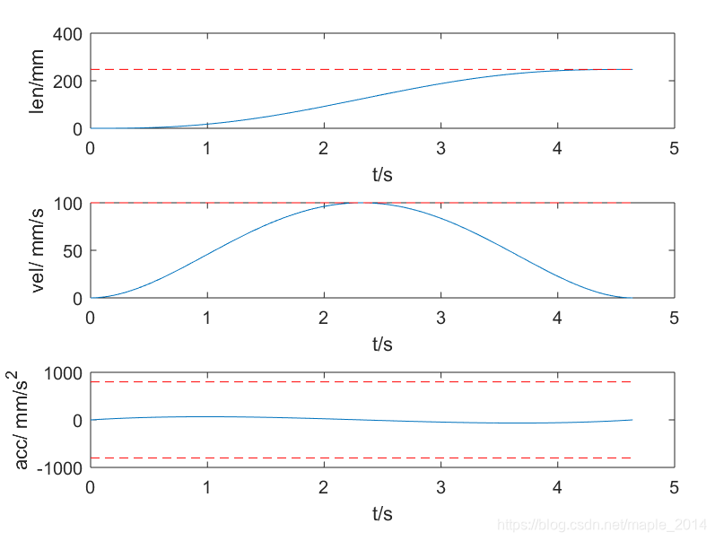
(4)速度规划(采用归一化五次多项式规划,详见博文:归一化5次多项式速度规划)
(5)直线插补
(6)计算每个插补点的逆运动学
(7)计算每个插补点的正运动学
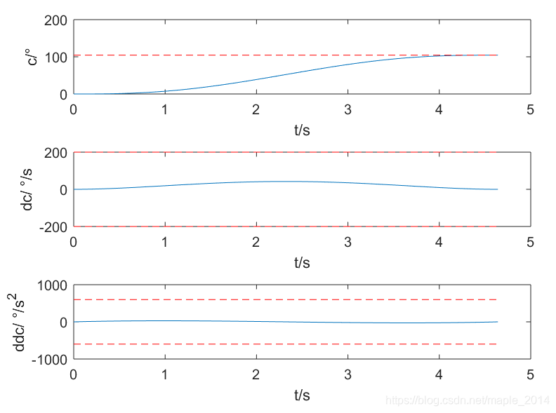
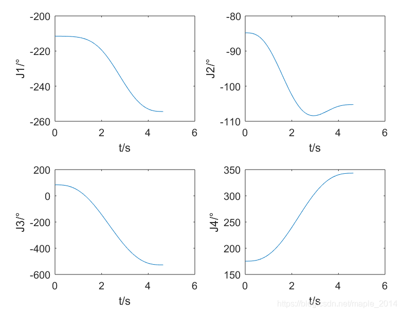
(8)画出直线插补结果,合成位置、速度、加速度,关节位置曲线,验证正逆解的正确性
四、MATLAB代码
%{
Function: find_handcoor
Description: 计算scara机器人当前手系
Input: 关节2角度theta2(rad)
Output: 机器人手系
Author: Marc Pony([email protected])
%}
function handcoor = find_handcoor( theta2 )
if (theta2 > 0.0 && theta2 < pi) || (theta2 > -2.0 * pi && theta2 < -pi)
    handcoor = 1;
else
    handcoor = 0;
end
end

%{
Function: find_flagJ1
Description: 计算scara机器人当前J1关节标志位
Input: 关节1角度theta1(rad)
Output: 机器人J1关节标志位flagJ1
Author: Marc Pony([email protected])
%}
function flagJ1 = find_flagJ1( theta1 )
if (theta1 >= -pi && theta1 <= pi)
    flagJ1 = 0;
else
    flagJ1 = 1;
end
end

%{
Function: find_flagJ2
Description: 计算scara机器人当前J2关节标志位
Input: 关节1角度theta2(rad)
Output: 机器人J2关节标志位flagJ2
Author: Marc Pony([email protected])
%}
function flagJ2 = find_flagJ2( theta2 )
if (theta2 >= -pi && theta2 <= pi)
    flagJ2 = 0;
else
    flagJ2 = 1;
end
end

%{
Function: scara_forward_kinematics
Description: scara机器人运动学正解
Input: 大臂长L1(mm),小臂长L2(mm),丝杆螺距screw(mm),机器人关节位置jointPos(rad)
Output: 机器人末端位置cartesianPos(mm或rad)
Author: Marc Pony([email protected])
%}
function cartesianPos = scara_forward_kinematics(L1, L2, screw, jointPos)
theta1 = jointPos(1);
theta2 = jointPos(2);
theta3 = jointPos(3);
theta4 = jointPos(4);
x = L1 * cos(theta1) + L2 * cos(theta1 + theta2);
y = L1 * sin(theta1) + L2 * sin(theta1 + theta2);
z = theta3 * screw / (2 * pi);
c = theta1 + theta2 + theta4;
cartesianPos = [x; y; z; c];
end

%{
Function: scara_inverse_kinematics
Description: scara机器人运动学逆解
Input: 大臂长L1(mm),小臂长L2(mm),丝杆螺距screw(mm),机器人末端坐标cartesianPos(mm或rad)
       手系handcoor,标志位flagJ1与flagJ2
Output: 机器人关节位置jointPos(rad)
Author: Marc Pony([email protected])
%}
function jointPos = scara_inverse_kinematics(L1, L2, screw, cartesianPos, handcoor, flagJ1, flagJ2)
x = cartesianPos(1);
y = cartesianPos(2);
z = cartesianPos(3);
c = cartesianPos(4);
jointPos = zeros(4, 1);

calculateError = 1.0e-8;
c2 = (x^2 + y^2 - L1^2 -L2^2) / (2.0 * L1 * L2);%若(x,y)在工作空间里,则c2必在[-1,1]里,但由于计算精度,c2的绝对值可能稍微大于1
temp = 1.0 - c2^2;

if temp < 0.0
    if temp > -calculateError
        temp = 0.0;
    else
        error('区域不可到达');
    end
end
if handcoor == 0    %left handcoor
    jointPos(2) = atan2(-sqrt(temp), c2);
else                %right handcoor
    jointPos(2) = atan2(sqrt(temp), c2);
end
s2 = sin(jointPos(2));
jointPos(1) = atan2(y, x) - atan2(L2 * s2, L1 + L2 * c2);
jointPos(3) = 2.0 * pi * z / screw;

if jointPos(1) <= -pi
    jointPos(1) = jointPos(1) + 2.0*pi;
end
if jointPos(1) >= pi
    jointPos(1) = jointPos(1) - 2.0*pi;
end

if flagJ1 == 1
    if jointPos(1) >= 0.0
        jointPos(1) = jointPos(1) - 2.0*pi;
    else
        jointPos(1) = jointPos(1) + 2.0*pi;
    end
end

if flagJ2 == 1
    if jointPos(2) >= 0.0
        jointPos(2) = jointPos(2) - 2.0*pi;
    else
        jointPos(2) = jointPos(2) + 2.0*pi;
    end
end
jointPos(4) = c - jointPos(1) - jointPos(2);
end

%{
Function: scara_shortest_path_inverse_kinematics
Description: scara机器人运动学逆解
Input: 大臂长L1(mm),小臂长L2(mm),丝杆螺距screw(mm),机器人末端坐标cartesianPos(mm或rad)
       手系handcoor,上一次的关节位置lastJointPos(rad)
Output: 机器人关节位置jointPos(rad)
Author: Marc Pony([email protected])
%}
function jointPos = scara_shortest_path_inverse_kinematics(len1, len2, screw, cartesianPos, handcoor, lastJointPos)
x = cartesianPos(1);
y = cartesianPos(2);
z = cartesianPos(3);
c = cartesianPos(4);
jointPos = zeros(4, 1);

calculateError = 1.0e-8;
c2 = (x^2 + y^2 - len1^2 -len2^2) / (2.0 * len1 * len2);%若(x,y)在工作空间里,则c2必在[-1,1]里,但由于计算精度,c2的绝对值可能稍微大于1
temp = 1.0 - c2^2;

if temp < 0.0
    if temp > -calculateError
        temp = 0.0;
    else
        error('区域不可到达');
    end
end
if handcoor == 0    %left handcoor
    jointPos(2) = atan2(-sqrt(temp), c2);
else                %right handcoor
    jointPos(2) = atan2(sqrt(temp), c2);
end
s2 = sin(jointPos(2));
jointPos(1) = atan2(y, x) - atan2(len2 * s2, len1 + len2 * c2);
jointPos(3) = 2.0 * pi * z / screw;

temp = zeros(3, 1);
for i = 1 : 2
    temp(1) = abs((jointPos(i) + 2.0*pi) - lastJointPos(i));
    temp(2) = abs((jointPos(i) - 2.0*pi) - lastJointPos(i));
    temp(3) = abs(jointPos(i) - lastJointPos(i));
    if temp(1) < temp(2) && temp(1) < temp(3)
        jointPos(i) = jointPos(i) + 2.0*pi;
    elseif temp(2) < temp(1) && temp(2) < temp(3)
        jointPos(i) = jointPos(i) - 2.0*pi;
    else
        %do nothing
    end
end
jointPos(4) = c - jointPos(1) - jointPos(2);
end
clc;
clear;
close all;

%% 输入参数
len1 = 200.0; %mm
len2 = 200.0; %mm
screw = 20.0; %mm
linearSpeed = 100; %mm/s
linearAcc = 800;   %mm/s^2
orientationSpeed = 200; %°/s
orientationAcc = 600;   %°/s^2
dt = 0.05; %s

%% 单点验证:
%(1)在[-2*pi, 2*pi]中随机生成4个关节角度(模拟示教过程)
%(2)计算标志位flagJ1和flagJ2,手系handcoor
%(3)计算正运动学
%(4)计算逆运动学
%(5)逆运动学结果与随机生成的关节角度作差,验证运动学正逆解的正确性
testCount = 1000000;
res = zeros(testCount, 4);
k = 1;
while k < testCount
    theta1 = -2.0*pi + 4.0*pi*rand;
    theta2 = -2.0*pi + 4.0*pi*rand;
    theta3 = -2.0*pi + 4.0*pi*rand;
    theta4 = -2.0*pi + 4.0*pi*rand;
    flagJ1 = find_flagJ1( theta1 );
    flagJ2 = find_flagJ2( theta2 );
    handcoor = find_handcoor( theta2 );
    jointPos = [theta1, theta2, theta3, theta4];
    cartesianPos = scara_forward_kinematics(len1, len2, screw, jointPos);

    jointPos2 = scara_inverse_kinematics(len1, len2, screw, cartesianPos, handcoor, flagJ1, flagJ2);
    res(k, :) = [theta1, theta2, theta3, theta4] - jointPos2';
    k = k + 1;
end
flag = all(abs(res - 0.0) < 1.0e-8) % flag = [1 1]则表示正逆解正确

while 1
    %% 直线验证:
    %(1)在[-2*pi, 2*pi]中随机生成4个关节角度,计算手系handcoor(模拟示教过程)
    %(2)运动学正解计算直线起点坐标(x,y,z,c)
    %(3)在工作空间里随机获取直线的终点x,y坐标,z在[-50mm,50mm]里随机生成,
    %   c在[-30°, 30°]里随机生成,手系与起点的相同(模拟示教过程)
    %(4)速度规划
    %(5)直线插补
    %(6)计算每个插补点的逆运动学
    %(7)计算每个插补点的正运动学
    %(8)画出直线插补结果,合成位置、速度、加速度,关节位置曲线,验证正逆解的正确性
    theta1 = -2.0*pi + 4.0*pi*rand;
    theta2 = -2.0*pi + 4.0*pi*rand;
    theta3 = -2.0*pi + 4.0*pi*rand;
    theta4 = -2.0*pi + 4.0*pi*rand;
    handcoor = find_handcoor( theta2 );
    jointPos = [theta1, theta2, theta3, theta4];
    cartesianPos = scara_forward_kinematics(len1, len2, screw, jointPos);
    lastJointPos = jointPos;
    x1 = cartesianPos(1);
    y1 = cartesianPos(2);
    z1 = cartesianPos(3);
    c1 = cartesianPos(4)*180.0/pi;

    figure(1)
    set(gcf, 'color','w');
    a = 0 : 0.01 : 2*pi;
    plot((len1 + len2)*cos(a), (len1 + len2)*sin(a), 'r--')
    hold on
    plot(x1, y1, 'ko')
    xlabel('x/mm');
    ylabel('y/mm');
    axis equal tight
    [x2, y2] = ginput(1);
    z2 = -50 + 50*rand;
    c2 = -30 + 60*rand;

    L = sqrt((x2 - x1)^2 + (y2 - y1)^2 + (z2 - z1)^2);
    C = abs(c2 - c1);
    T = max([1.875 * L / linearSpeed, 1.875 * C / orientationSpeed, ...
        sqrt(5.7735 * L / linearAcc), sqrt(5.7735 * C / orientationAcc)]);

    t = (0 : dt : T)';
    u = t / T;
    if abs(t(end) - T) > 1.0e-8
        t = [t; T];
        u = [u; 1];
    end
    u = t / T;
    s = 10*u.^3 - 15*u.^4 + 6*u.^5;
    ds = 30*u.^2 -60*u.^3 + 30*u.^4;
    dds = 60*u - 180*u.^2 + 120*u.^3;

    len = L * s;
    vel = (L / T) * ds;
    acc = (L / T^2) * dds;
    pos = zeros(length(t), 4);
    jointPos = zeros(length(t), 4);
    cartesianPos = zeros(length(t), 4);
    rate = [x2 - x1, y2 - y1, z2 - z1, c2 - c1] / L;
    for i = 1 : length(t)
        pos(i, :) = [x1, y1, z1, c1] + len(i) * rate;
        pos(i, 4) = pos(i, 4)*pi/180.0;
        jointPos(i, :) = scara_shortest_path_inverse_kinematics(len1, len2, screw, pos(i, :), handcoor, lastJointPos);
        cartesianPos(i, :) = scara_forward_kinematics(len1, len2, screw, jointPos(i, :));
        lastJointPos = jointPos(i, :);
    end
    plot3(cartesianPos(:, 1), cartesianPos(:, 2), cartesianPos(:, 3), 'ro');
    plot3([x1 x2], [y1 y2], [z1 z2], '+','markerfacecolor','k','markersize', 14)

    figure(2)
    set(gcf, 'color','w');
    subplot(3,1,1)
    plot(t, len)
    hold on
    plot([0 t(end)], [L L], 'r--')
    xlabel('t/s');
    ylabel('len/mm');
    subplot(3,1,2)
    plot(t, vel)
    hold on
    plot([0 t(end)], [linearSpeed linearSpeed], 'r--')
    xlabel('t/s');
    ylabel('vel/ mm/s');
    subplot(3,1,3)
    plot(t, acc)
    hold on
    plot([0 t(end)], [linearAcc linearAcc], 'r--')
    plot([0 t(end)], [-linearAcc -linearAcc], 'r--')
    xlabel('t/s');
    ylabel('acc/ mm/s^2');

    figure(3)
    set(gcf, 'color','w');
    subplot(3,1,1)
    plot(t, len*rate(4))
    hold on
    plot([0 t(end)], [c2-c1 c2-c1], 'r--')
    xlabel('t/s');
    ylabel('c/°');
    subplot(3,1,2)
    plot(t, vel*rate(4))
    hold on
    plot([0 t(end)], [orientationSpeed orientationSpeed], 'r--')
    plot([0 t(end)], [-orientationSpeed -orientationSpeed], 'r--')
    xlabel('t/s');
    ylabel('dc/ °/s');
    subplot(3,1,3)
    plot(t, acc*rate(4))
    hold on
    plot([0 t(end)], [orientationAcc orientationAcc], 'r--')
    plot([0 t(end)], [-orientationAcc -orientationAcc], 'r--')
    xlabel('t/s');
    ylabel('ddc/ °/s^2');

    figure(4)
    set(gcf, 'color','w');
    subplot(2,2,1)
    plot(t, jointPos(:,1)*180.0/pi)
    xlabel('t/s');
    ylabel('J1/°');
    subplot(2,2,2)
    plot(t, jointPos(:,2)*180.0/pi)
    xlabel('t/s');
    ylabel('J2/°');
    subplot(2,2,3)
    plot(t, jointPos(:,3)*180.0/pi)
    xlabel('t/s');
    ylabel('J3/°');
    subplot(2,2,4)
    plot(t, jointPos(:,4)*180.0/pi)
    xlabel('t/s');
    ylabel('J4/°');

    pause()
    close all
end