SVM
1.Introduction
Support vector machine is highly preferred by many as it produces significant accuracy with less computation power. Support Vector Machine, abbreviated as SVM can be used for both regression and classification tasks. But, it is widely used in classification objectives.
The objective of the support vector machine algorithm is to find a hyperplane in an N-dimensional space(N — the number of features) that distinctly classifies the data points.To separate the data points, there are many possible hyperplanes that could be chosen. Our objective is to find a plane that has the maximum margin, i.e the maximum distance between data points of both allclasses. Maximizing the margin distance provides some reinforcement so that future data points can be classified with more confidence.
2.Hyperplanes and Support Vectors
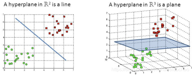
Hyperplanes are decision boundaries that help classify the data points. Data points falling on either side of the hyperplane can be attributed to different classes.
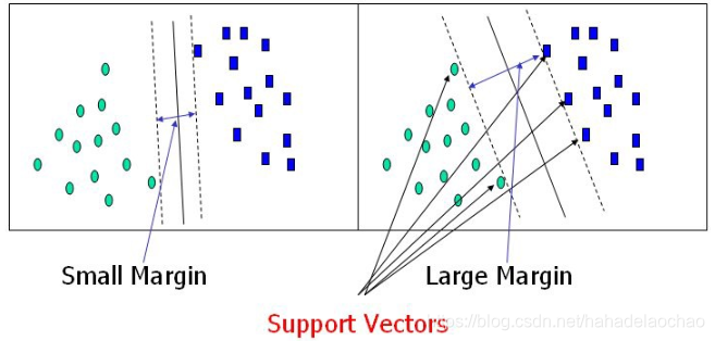
Support vectors are data points that are closer to the hyperplane and influence the position and orientation of the hyperplane. Using these support vectors, we maximize the margin of the classifier.
3.Large Margin
In logistic regression, we take the output of the linear function and squash the value within the range of [0,1] using the sigmoid function. If the squashed value is greater than a threshold value(0.5) we assign it a label 1, else we assign it a label 0. In SVM, we take the output of the linear function and if that output is greater than 1, we identify it with one class and if the output is -1, we identify is with another class. Since the threshold values are changed to 1 and -1 in SVM, we obtain this reinforcement range of values([-1,1]) which acts as margin.
4.Hard-margin
We are given a training dataset of {\displaystyle n}n points of the form

where the y_{i} are either 1 or −1, each indicating the class to which the point{\vec {x}}{i} belongs. Each{\vec {x}}{i} is a p-dimensional real vector. We want to find the “maximum-margin hyperplane” that divides the group of points {\vec {x}}{i} for which{ y{i}=1} from the group of points for which {y_{i}=-1}, which is defined so that the distance between the hyperplane and the nearest point {\vec {x}}{i} from either group is maximized.
hyperplane can be written as the set of points {\vec {x}} satisfying
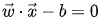
If the training data is linearly separable, we can select two parallel hyperplanes that separate the two classes of data, so that the distance between them is as large as possible. The region bounded by these two hyperplanes is called the “margin”, and the maximum-margin hyperplane is the hyperplane that lies halfway between them. With a normalized or standardized dataset, these hyperplanes can be described by the equations.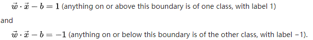
The distance is computed using the distance from a point to a plane equation. We also have to prevent data points from falling into the margin, we add the following constraint: for each i either:
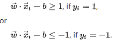
These constraints state that each data point must lie on the correct side of the margin.
This can be rewritten as:

5.Soft-margin
To extend SVM to cases in which the data are not linearly separable, we introduce the hinge loss function.

This function is zero if {x}}{i} lies on the correct side of the margin. For data on the wrong side of the margin, the function’s value is proportional to the distance from the margin.
We then wish to minimize:

where the parameter lambda determines the trade-off between increasing the margin size and ensuring that the{\vec {x}}_{i} lie on the correct side of the margin. Thus, for sufficiently small values of lambda , the second term in the loss function will become negligible, hence, it will behave similar to the hard-margin SVM, if the input data are linearly classifiable, but will still learn if a classification rule is viable or not.
By solving for the Lagrangian dual of the above problem, one obtains the simplified problem:
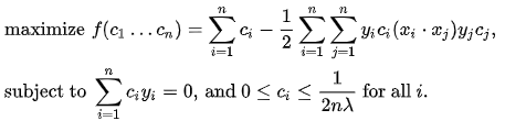
This is called the dual problem. Since the dual maximization problem is a quadratic function of the c_i subject to linear constraints, it is efficiently solvable by quadratic programming algorithms.

6.Kernel trick
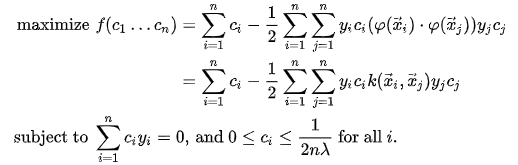
Suppose now that we would like to learn a nonlinear classification rule which corresponds to a linear classification rule for the transformed data points.
Moreover, we are given a kernel function k which satisfies :

Support-vector machine

猜你喜欢
转载自blog.csdn.net/hahadelaochao/article/details/105610296
今日推荐
周排行