Machine Learning in Action(6) —— Support Vector Machine

Machine Learning in Action(6) —— Support Vector Machine

 

1.Difference between logistic regression and Support Vector Machine

 

• Logistic regression:

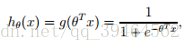
hypothesis:

one vector θ is the parameter we want to fit.

g(z):

Here, g(z) = 1 if z>=0, and g(z) = 0 otherwise.

Convention:  x0=1

The class label is 0 or 1

 

• Support Vector Machine:

Hypothesis:

two vectors w, b are the parameters we want to fit.

[g(z)]

Here ,g(z) = 1 if z>=0, and g(z) = -1 otherwise.

Drop the convention of x0=1. Instead, b takes the role of what was previously θ0   , and w takes the role of [θ1, θ2, ……]T.

The class label is -1 or 1.

 

The value of the class label depends on the value of g(z).

 

2.Margins

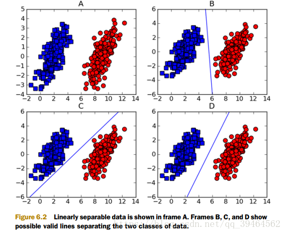
• What is linearly separable ?

It means that we can separate a dataset with a straight line

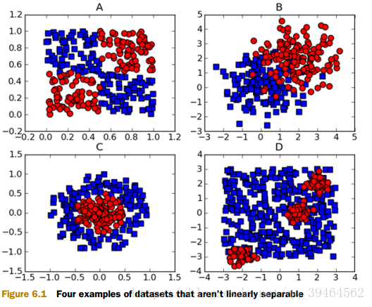
Examples about linearly separable dataset:

 

Examples that are not linearly separable:

• What is hyperplane?

For the linearly separable dataset, all the examples are divided into two parts by a straight line, which is called decision boundary, also called separating hyperplane . This line can be described by two parameters slope and intercept . Moreover, for the following discussion about support vector machine algorithm, this hyperplane has the form:  WT + b = 0.

 

• What is the confidence of predication?

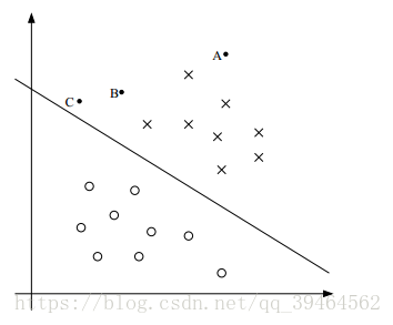
In the figure above, we can see that this dataset is linearly separable and the straight line in the figure is the separating hyperplane, and there are there points A,B, and C. And A is far away from the hyperplane but C is very close to the hyperplane. If we are asked to make a predication for the class label at A, we should be quite confident that the label is x . However, if we are asked to make a predication at point C, we can’t be quite sure its label is x, because it seems that just a small change to the hyperplane will cause our predication changed.

 

Thus , for linearly separable dataset, if a point is far from the hyperplane, then we may be significantly more confident in our predication.

 

Take the logistic regression to explain:

the step function is g(z):

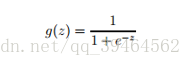
it’s a function like this:

 

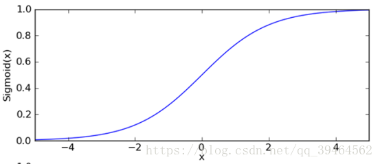
And our hypothesis is:

Combining the hypothesis and the plot of sigmoid function,  we can see that if

ΘT X>>0, there is a great probability that y=1, similarly, if ΘT X <<0, we can quite sure that y=0.

 

Thus our goal is to make a very confident predication for a new data.

 

Now the problem is: how to describe the confidence of a predication?
 

Before describing the confidence of the predication, we should know two definitions first.

 

• Functional margin

 

Functional margin for one training example :

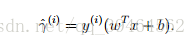
Given a training example (x(i), y(i)), we define the functional margin of (w, b) with respect to the training example as (gamma hat) :

Note that the separating hyperplane is the line: WT + b = 0, so if WT + b > 0, it means the point is at the top right of the hyperplane, otherwise it’s at the lower left of the hyperplane. In addition, according to our hypothsis, if WT + b > 0, y = 1, so the functional margin is a positive number, if WT + b < 0 , y=-1, the functional mragin is also a positive number.

 

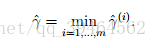
Functional margin for the whole training set :

Given a training set S = {(x(i), y(i)); i = 1, . . . , m}, we also define the function margin of (w, b) with respect to S to be the smallest of the functional margins of the individual training examples. Denoted by ˆ γ, this can therefore be written:

 

 

• Geometric margin

 

Geometric margin for one training example:

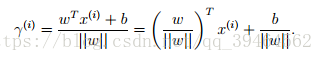
Consider the point A, its distance to the decision boundary, r(i), is given by the line segment AB, AB = r(i).  r(i) (gamma)is called the geometric margin.

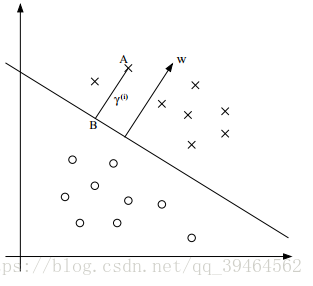
For the picture above, the decision boundary is shown, and it’s must be the case that our vector w is orthogonal to the separating hyperplane. Thus, w/||w|| is a unit-length vector.

Point A represents the input x(i) of some training example with label y(i)=1

So the point B is given by x(i) – r(i) * w/||w||. (Keep mind that x(i) is actually a vector with some features)

Also because point B lies on the decision boundary, so it must satisfy the equation WT + b = 0, hence,

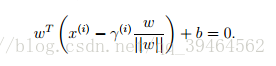
And we can solve for r(i) through the equation above:

 

 

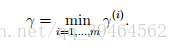
Geometric margin for the whole training set:

given a training set S = {(x(i), y(i)); i = 1, . . . , m}, we also define the geometric margin of (w, b) with respect to S to be the smallest of the geometric margins on the individual training examples:

 

Note that if ||w|| = 1, then functional margin equals geometric margin.

 

Knowing the definition of functional and geometric margin, we can try to describe the confidence of predication

.

• First attempt to describe the confidence of our predication —— functional margin

We use the function margin:

For one example:

For whole training set:  

to measure the confidence of our predication. A large functional margin represents a confident and correct predication.

 

• Second attempt to describe the confidence of our predication —— modified functional margin

 

Actually, it’s not true that the bigger the functional margin is, the higher the reliability of the predication is. Because by exploiting our freedom to scale w and b, we can make the functional margin arbitrarily large without really changing anything meaningful.

So we should add some conditions to the functional margin:

First one:

make || w || = 1 and then we might replace (w, b) with (w/||w||, b/||w||), and instead consider the functional margin of (w/||w||, b/||w||).

 

• Third attempt to describe the confidence of our predication —— geometric margin

 

It’s a natural desideratum that the farther the distance between decision boundary and the data point, the more confident we are for the predication we make. The geometric margin is just that distance. Thus, we describe the confidence of our predication by the geometric margin.

For one example:

For whole training set:

 

The decision boundary with the maximal geometric margin will make the most credible predication.   

 

 

Note that unlike the functional margin the geometric margin is invariant to rescaling of the parameters w and b; i.e., if we replace w with 2w and b with 2b, then the geometric margin does not change.

 

3. Optimal margin classifier —— use the third way (geometric margin)to describe the confidence of our predication

 

If we can find a decision boundary that maximizes the geometric margin, this will reflect a very confident set of predications on the training set and a good “fit” to the training data.

In addition, this will result in a classifier that separates the positive and negative training examples with the maximal geometric margin(maximal  “gap”).

 

This classifier is called the optimal margin classifier

 

 

Now the problem is to find that hyperplane and get an optimal margin classifier.

 

 

4. Formalize the optimization problem

 

Assumption: our training set is linearly separable

Goal:

# first attempt—— add a constraint about ||w||

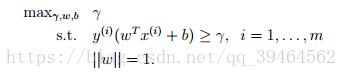
We want to maximize γ, subject to each training example having functional margin(the definition of functional margin for each example is y(i)(wTx(i) + b)) at least γ . Moreover, the constraint ||w||=1 ensures that the functional margin equals to geometric margin, so we can also guarantee that the geometric margin is at least γ. Thus, solving this problem we ‘ll get an optimal classifier with the largest possible geometric margin with respect to the training set (but not the one single example).

 

Problem: constraint ||w|| = 1 is a nasty (non-convex) one, which causes it’s very difficult to solve this optimization problem.

 

# second attempt —— get rid of the constraint ||w||=1

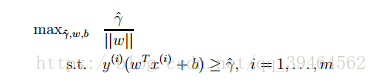
We are going to maximize ˆ γ/||w|| , subject to the functional margin all being at least ˆ γ . Since the geometric and functional margins are related by

γ = ˆ γ/||w|. Solving this problem will also result in an optimal classifier with the largest possible geometric margin.

 

Problem:

Although we get rid of the nasty constraint, we now have a nasty objective

ˆ γ/||w||  function.

 

# third attempt —— add a scaling constraint for the second attempt

 

We add a constraint:

For geometric margin, we can add an arbitrary scaling constraint without changing anything, so we can satisfy this constraint(functional margin=1) by rescaling our parameters w and b.
 

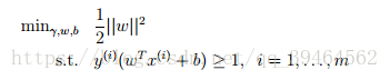
With this constraint, our objective function above becomes maximizing 1/||w||, which the same thing as minimizing ||w||2

 

Thus, the ultimate form of our optimization problem is:

Now, this optimization problem with a convex quadratic objective and only linear constraints can be efficiently solved. Its solution gives us the optimal margin classifier.

 

Now the problem is how to solve this constrained optimization problem —— we can turn to the Lagrange multipliers.

 

5. Lagrange duality

 

• Optimization problem with only equality constraint

Lagrange multipliers can be used to solve the constrained optimization problem. The problem can be of the following form:

We want to find parameter w that minimize the function f(w) and satisfying some constraints hi(w)=0, i = 1, ……, l.

 

Use the Lagrange multipliers to solve this constrained optimization problem.

 

Define the Lagrangian to:

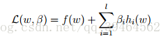
bi’s are called Lagrange multipliers.

To find the parameter w that can optimize this problem, we can just set L’s partial derivatives to zero:

 

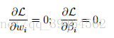
and solve for w and b.

 

• Generalized optimization problem with inequality constraints as well as equality constraints.

 

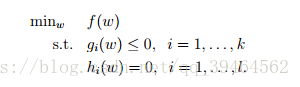
     （1）Primal optimization problem:

 

Definition of primal optimization problem:

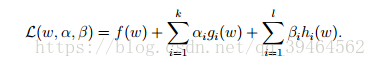
Generalized Lagrangian:

αi’s and βi’s are called the Lagrange multipliers.

 

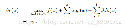
Define a quality:

  

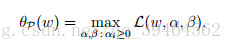
Note that we are maximizing with respect to α and β but not w.

 

Some cool thing about this equality and our primal optimization problem:

 

Let some w be given. If w violates any of the primal constraints (i.e., if either gi(w) > 0 or hi(w) 6= 0 for some i), then we are able to verify that:

Conversely, if the constraints are indeed satisfied for a particular value of w, then θP(w) = f(w). Hence,

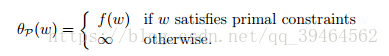
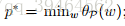
Thus, θP takes the same value as the objective in our problem for all values of w that satisfies the primal constraints, and is positive infinity if the constraints are violated. Hence, if we consider the minimization problem:

 

(Note that we have the constraint that αi > 0)

we see that it is the same problem (i.e., and has the same solutions) as our original, primal problem.

 

We define a notation p* as the optimal value of primal problem. That is :

 

 

     （2）Dual optimization problem

 

Define another quality similar to θp(w):

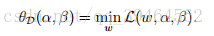
Note that for this quality we are minimizing with respect to w but not α and β.

 

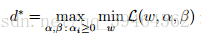
Definition of dual optimization problem with the quality above:

 

 

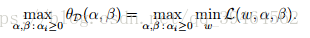
We define a notation d* as the optimal value of the dual optimization problem, that is:

 

   （3）Relation between the primal optimization problem and the dual optimization problem (or relation between p* and d*)

(we use the rule that the “max min” of a function is always less than the “min max” of a function)

 

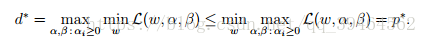
Thus, under certain conditions, we’ll have:

d* = p*,

 

so in this case, we can solve the dual optimization problem in lieu of the primal problem.

 

Now the problem is what are the certain conditions?

 

Assumptions:

• f(w):  convex
• gi(w):  convex & feasible(there exists some w so that gi(w)<0 for all i)
• hi(w):  affine

 

inference:

• there exists w*, α* and β* so that w* is the solution to the primal problem, α* and β* are the solution to the dual problem.
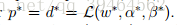
• Moreover, w* , α* and β* satisfy the equation:

• Moreover, w* , α* and β* also satisfy the KKT(Karush-Kuhn-Tucker ) conditions, which are as follows:

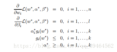
• Moreover, if some w* , α* and β* satisfy the KKT conditions, then it is also a solution to the primal and dual problems.
• Moreover, the third equation in the KKT conditions are called the dual complementarity condition. Specifically, it implies that if

αi*>0, then gi(w*)=0 (i.e., constraint “gi(w) <=0” is active, meaning it holds with equality rather than with inequality)

 

 

 

6. Definition of Support Vector

 

Before we talked about the generalized Lagrange, primal optimization problem and dual optimization problem, we’ve formalized the optimal margin classifier, and the ultimate form is:

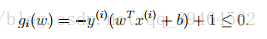
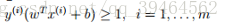
In order to make use of the generalized Lagrange and the relation between primal and dual optimization problem, we can write the constraint as:

From the KKT dual complementarity condition, we’ll have αi > 0 only for training examples that have gi(w) exactly equal to 0, and that means term y(i)(wTx(i) + b) exactly equals to 1. Notice that the term y(i)(wTx(i) + b) is just the functional margin of a training example.

 

Thus, we have a conclusion that we will have αi > 0 only for the training examples that have functional margin exactly equal to 1.

 

If gi(w) !=0, according to the constraint, then gi(w) <0, in other words, functional margin is greater than 1. Moreover, in most cases, if gi(w) !=0, then αi = 0 (KKT dual complementarity condition).

Thus, we have another conclusion that we will have αi = 0 for the training examples that have functional margin greater than 1.(in most cases but not all the cases.)

 

 

Combined the two conclusions we made above, we can know that the points with the smallest margins are exactly the ones closest to the decision boundary. And for a training set, the smallest functional margin is 1. Moreover for these points αi  > 0. So for the other points that have the further distance, their αi’s in most cases are 0s. Like the figure below:

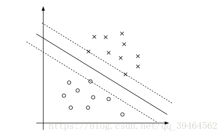
And those closest points are called support vectors.

 

Moreover, it’s obvious that the number of support vectors can be much smaller than the size of the training set because the number of points that is the closest to the decision boundary is small. (As shown in the figure above.)

 

 

 

7. Solving our optimization problem with Lagrange multipliers and relation between primal problem and dual problem.

 

The form of our optimization problem:

Thus, f(w) = ||w||2 /2;

We can write the inequality constraint as:

 

（1）Construct Lagrangian (called L1):

 

 (1)

 

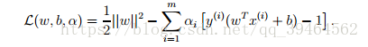
Comparing to the generalized Lagrangian (called L2)

We can find that for L1, w and b are two parameters and α is a Lagrange multiplier because it has only one inequality constraint, while for L2, w is a parameter and α, β are two Lagrange multipliers because the generalized Lagrangian has both inequality constraint and equality constraint.

 

（2）Find the dual problem for our primal optimization problem:

 

• First, get θD(α) :

θD(α) = min L(w, b, α) with respect to w and b.

To minimize L(w, b, α), we set the derivatives of L with respect to w and b to zero:

 

Derivative with respect to w:

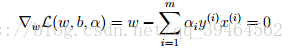
which implies:

   (2)

 

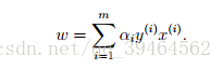
Derivative with respect to b:

 (3)

 

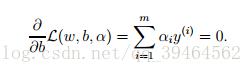
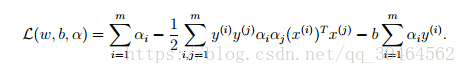
If we take the definition of w in equation (2) and plug that back into the Lagrangian(equation(1)) and simplify, we get:

 

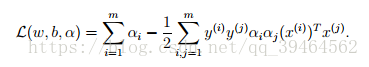
But from equation(3), the last term in the Lagrangian must be 0, so we obtain:

 

 

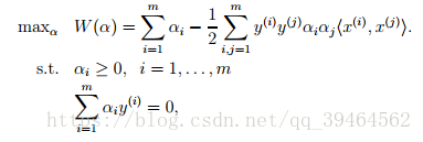
• Second, define the dual optimization problem:

 

 

Conditions required for p*=d* and the KKT conditions are indeed satisfied in this dual optimization problem. So we can solve the dual in lieu of solving the primal problem.

 

 

（3）Solve the dual optimization problem:

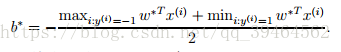
Until now our goal is to find the α’s (α*)that maximize the W(α) subject to the constraints. And then we use equation(2) to go back and find the optimal w’s(w*) as a function of α’s. And next having found w*, by consider the primal problem, we can find the value of the intercept term b as:

.

 

（4）Make predication use the parameters we’ve found:

Up to now we’ve fit our model’s parameters (w*, α*, b*) to the training set, so we can make a predication at a new point input x by calculating wT x +b and predict y = 1 if and only if b this quantity is bigger than zero.

 

8. Recap

 

The process that we get the ultimate form of our optimization problem:

 

First , three attempts were made to describe the confidence of predication, and finally we decided to describe it with the geometric margin;

Next, with the description of the confidence, we attempted to formalized the optimization problem for three times, and finally we get the ultimate form:

Third attempt:

Add a constraint: (functional margin = 1)

 

ultimate form:  

constraint:

 

 

The process of solving the optimization problem:

 

First, we learn the Lagrange multiplier and the generalized Lagrange.

Second, we find the relationship between primal optimization problem and dual optimization problem.

Third, we define the support vectors.

Then, we take the ultimate form of our optimization problem above as the primal problem

Next, construct the dual problem for primal problem

Next, solve the dual optimization problem and get the parameters w and b in in wT + b = 0.

Finally we can make predication using the parameters in the last step.