【机器学习】线性回归

1. 问题

假设你是一个餐饮连锁店的CEO，你打算在不同的城市开设不同的分店。你已经在一些城市开了分店而且你有这些城市人口与利润的数据（见 5. 数据 data.txt），你希望通过这些数据来决定在哪些城市新开分店（也就是通过新城市的人口预测新城市的利润）。

2. 解决

线性回归

假设利润与 人口数 的函数关系为： $h_{\theta}(x) = \theta_0 + \theta_1x$

实现了单变量线性回归模型，且仅针对单变量线性回归有效.

实现时为使最小化代价函数 $J(\theta) = \frac{1}{2m}\sum_{i=1}^m (h_{\theta}(x^{(i)})-y^{(i)})^2$ （均方误差），使用梯度下降法获得线性回归参数。

在这里插入图片描述
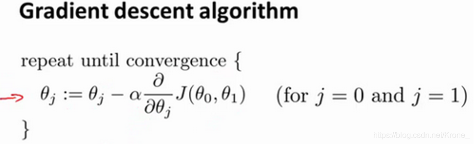
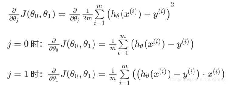
代价函数的导数：

需要设置的初始参数有 $\theta_0$ 、 $\theta_1$ 、学习率 $\alpha$ 。

$\theta_0 = 0$
$\theta_1 = 0$
$\alpha = 0.01$

终止条件采用了两种方法（两种方法中任意一个满足条件时迭代终止）：

迭代步数限制（ $STEP = 10000$ ）
当两次迭代获得的差异（ $\Delta = 0.0000001$ ）较小时终止迭代

3. 代码

import pandas as pd
import matplotlib.pyplot as plt
import numpy as np
from pylab import mpl

mpl.rcParams['font.sans-serif'] = ['FangSong'] # 指定默认字体
mpl.rcParams['axes.unicode_minus'] = False # 解决保存图像是负号'-'显示为方块的问题

# 假设：单变量线性回归
def hypothesis(x, theta0, theta1):
    return theta0 + theta1 * x
# 代价函数(Cost function)：
def CostFunction(X, Y, theta0, theta1):
    m = np.shape(X)[0]
    res = 1
    for i in range(m):
        res += pow(hypothesis(X[i], theta0, theta1) - Y[i], 2)
    res /= (2*m)
    return res
# 代价函数的导数
def CostFunction_derivative(j, X, Y, theta0, theta1):
    m = np.shape(X)[0]
    res = 0
    for i in range(m):
        tmp = hypothesis(X[i], theta0, theta1) - Y[i]
        if j == 1:
            tmp *= X[i]
        res += tmp
    res /= m
    return res
# 批量梯度下降算法
def gradientDescent(X, Y, theta0, theta1, a):
    temp0 = theta0 - a * CostFunction_derivative(0, X, Y, theta0, theta1)
    temp1 = theta1 - a * CostFunction_derivative(1, X, Y, theta0, theta1)
    return temp0, temp1
# 绘制二维散点图
def plot_data(X, Y, title, xlabel, ylabel):
	plt.plot(X, Y, 'ro', markersize=6)
	plt.title(title, fontsize=20)
	plt.xlabel(xlabel, fontsize=10)
	plt.ylabel(ylabel, fontsize=10)
	plt.ioff() # 使matplotlib的显示模式转换为交互（interactive）模式


# 读取数据
dataset = pd.read_csv('data1a.txt', header=None) # 设置header参数，读取文件的时候没有标题
X = dataset.iloc[:,0].values # 人口数
Y = dataset.iloc[:,1].values # 利润

# 参数 θ 初始化
theta0 = 0
theta1 = 0

# 学习率
learningRate = 0.01

# 循环终止条件设定
STEP = 10000 # 设定一个比较大的迭代步数。
Delta = 0.0000001 # 当两次迭代获的J(θ) 差异较小时终止迭代。

if __name__ == '__main__':
    cnt = 0
    Jlast = 0
    Jnow = CostFunction(X, Y, theta0, theta1)
    Jlist = [Jnow]
    while cnt < STEP and abs(Jnow - Jlast) > Delta:
        theta0, theta1 = gradientDescent(X, Y, theta0, theta1, learningRate);
        # print(theta0, theta1)
        Jlast = Jnow
        Jnow = CostFunction(X, Y, theta0, theta1)
        Jlist.append(Jnow)
        cnt += 1
    print("梯度下降法获得线性回归参数")
    print("θ0 = ", theta0)
    print("θ1 = ", theta1)
    print()
    print("回归模型在所有训练数据（train_data.txt）上最终的J(θ)值")
    print("J(θ) = ", Jnow)
    print()
    # 画图
    plt.figure(figsize=(10, 6))
    # figure = plt.subplot(211)
    plt.plot(Jlist)
    plt.xlabel(u'迭代步数')
    plt.ylabel(u'代价函数值J(θ)')
    plt.title(u'J(θ)随迭代步数的变化')

    plt.figure(figsize=(10, 6))
    # plt.subplot(212)
    plt.scatter(X, Y, color='red')
    plt.plot(X, predict, color='black')
    plt.xlabel(u'人口数')
    plt.ylabel(u'利润')
    plt.title(u'线性回归')
    plt.show()

4. 结果

梯度下降法获得线性回归参数：
$\theta_0 = -3.8783681899109235$
$\theta_0 = 1.1912843507674498$

回归模型在所有训练数据（data.txt）上最终 $J(θ) = 4.482153618457505$

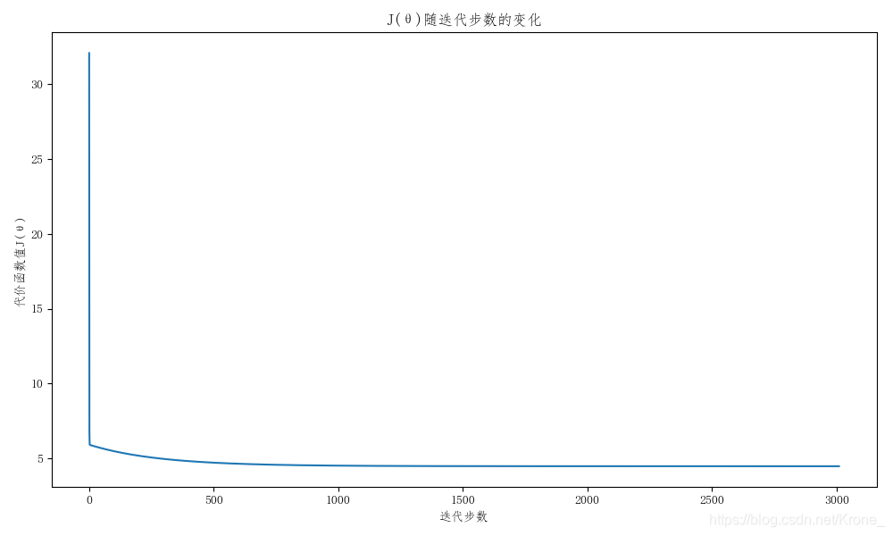
循环过程中 $J(\theta)$ 随迭代步数变化的图
在这里插入图片描述
线性回归的拟合效果

5. 数据

data.txt

6.1101,17.592
5.5277,9.1302
8.5186,13.662
7.0032,11.854
5.8598,6.8233
8.3829,11.886
7.4764,4.3483
8.5781,12
6.4862,6.5987
5.0546,3.8166
5.7107,3.2522
14.164,15.505
5.734,3.1551
8.4084,7.2258
5.6407,0.71618
5.3794,3.5129
6.3654,5.3048
5.1301,0.56077
6.4296,3.6518
7.0708,5.3893
6.1891,3.1386
20.27,21.767
5.4901,4.263
6.3261,5.1875
5.5649,3.0825
18.945,22.638
12.828,13.501
10.957,7.0467
13.176,14.692
22.203,24.147
5.2524,-1.22
6.5894,5.9966
9.2482,12.134
5.8918,1.8495
8.2111,6.5426
7.9334,4.5623
8.0959,4.1164
5.6063,3.3928
12.836,10.117
6.3534,5.4974
5.4069,0.55657
6.8825,3.9115
11.708,5.3854
5.7737,2.4406
7.8247,6.7318
7.0931,1.0463
5.0702,5.1337
5.8014,1.844
11.7,8.0043
5.5416,1.0179
7.5402,6.7504
5.3077,1.8396
7.4239,4.2885
7.6031,4.9981
6.3328,1.4233
6.3589,-1.4211
6.2742,2.4756
5.6397,4.6042
9.3102,3.9624
9.4536,5.4141
8.8254,5.1694
5.1793,-0.74279
21.279,17.929
14.908,12.054
18.959,17.054
7.2182,4.8852
8.2951,5.7442
10.236,7.7754
5.4994,1.0173
20.341,20.992
10.136,6.6799
7.3345,4.0259
6.0062,1.2784
7.2259,3.3411
5.0269,-2.6807
6.5479,0.29678
7.5386,3.8845
5.0365,5.7014
10.274,6.7526
5.1077,2.0576
5.7292,0.47953
5.1884,0.20421
6.3557,0.67861
9.7687,7.5435
6.5159,5.3436
8.5172,4.2415
9.1802,6.7981
6.002,0.92695
5.5204,0.152
5.0594,2.8214
5.7077,1.8451
7.6366,4.2959
5.8707,7.2029
5.3054,1.9869
8.2934,0.14454
13.394,9.0551
5.4369,0.61705

Krone_

发布了76 篇原创文章 · 获赞 20 · 访问量 2万+

私信关注