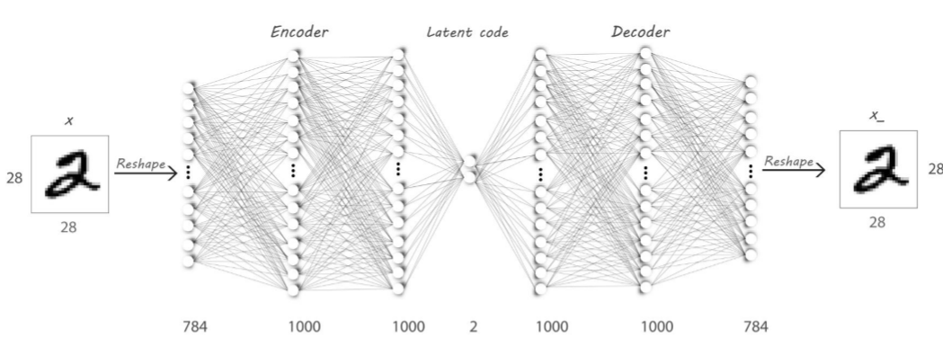
1、Auto-Encoder
降到自定义层
  1 import  os
  2 import  tensorflow as tf
  3 import  numpy as np
  4 from    tensorflow import keras
  5 from    tensorflow.keras import Sequential, layers
  6 from    PIL import Image
  7 from    matplotlib import pyplot as plt
  8
  9
 10
 11 tf.random.set_seed(22)
 12 np.random.seed(22)
 13 os.environ['TF_CPP_MIN_LOG_LEVEL'] = '2'
 14 assert tf.__version__.startswith('2.')
 15
 16
 17 def save_images(imgs, name): #将多张image保存为一张image
 18     new_im = Image.new('L', (280, 280))
 19
 20     index = 0
 21     for i in range(0, 280, 28):
 22         for j in range(0, 280, 28):
 23             im = imgs[index]
 24             im = Image.fromarray(im, mode='L')
 25             new_im.paste(im, (i, j))
 26             index += 1
 27
 28     new_im.save(name)
 29
 30
 31 h_dim = 20  #将原来的784维的数据降到20维数据,任意设定
 32 batchsz = 512 #
 33 lr = 1e-3  #学习率
 34
 35
 36 (x_train, y_train), (x_test, y_test) = keras.datasets.fashion_mnist.load_data()
 37 x_train, x_test = x_train.astype(np.float32) / 255., x_test.astype(np.float32) / 255.
 38 # 不需要labels,所以不加载y
 39 train_db = tf.data.Dataset.from_tensor_slices(x_train)
 40 train_db = train_db.shuffle(batchsz * 5).batch(batchsz)
 41 test_db = tf.data.Dataset.from_tensor_slices(x_test)
 42 test_db = test_db.batch(batchsz)
 43
 44 print(x_train.shape, y_train.shape)
 45 print(x_test.shape, y_test.shape)
 46
 47
 48
 49 class AE(keras.Model): #继承keras.Model
 50
 51     def __init__(self):
 52         super(AE, self).__init__()
 53
 54         # Encoders  3层全连接层,输入维度为28x28,784
 55         self.encoder = Sequential([
 56             layers.Dense(256, activation=tf.nn.relu),
 57             layers.Dense(128, activation=tf.nn.relu),
 58             layers.Dense(h_dim)  #降到自定义维度
 59         ])
 60
 61         # Decoders 输入维度为h_dim,3个全连接层,升到高维
 62         self.decoder = Sequential([
 63             layers.Dense(128, activation=tf.nn.relu),
 64             layers.Dense(256, activation=tf.nn.relu),
 65             layers.Dense(784)
 66         ])
 67
 68
 69     def call(self, inputs, training=None):  #前向传播过程
 70         # [b, 784] => [b, 10] 降维
 71         h = self.encoder(inputs)
 72
 73         # [b, 10] => [b, 784] 重建
 74         x_hat = self.decoder(h)
 75
 76         return x_hat
 77
 78
 79
 80 model = AE()  #创建模型
 81 model.build(input_shape=(None, 784)) #这里要使用元组类型进行传入
 82 model.summary()
 83
 84 optimizer = tf.optimizers.Adam(lr=lr)  #优化器
 85
 86
 87 for epoch in range(100):
 88     for step, x in enumerate(train_db):
 89
 90         #先进行reshape,[b, 28, 28] => [b, 784]
 91         x = tf.reshape(x, [-1, 784])
 92
 93         with tf.GradientTape() as tape:  #梯度器,用来写要求梯度的函数
 94             x_rec_logits = model(x)
 95
 96             rec_loss = tf.losses.binary_crossentropy(x, x_rec_logits, from_logits=True)  #将图片的每一个点都当作一个分类问题
 97             rec_loss = tf.reduce_mean(rec_loss)  # 求均值
 98
 99         grads = tape.gradient(rec_loss, model.trainable_variables)
100         optimizer.apply_gradients(zip(grads, model.trainable_variables))
101
102
103         if step % 100 ==0:
104             print(epoch, step, float(rec_loss))
105
106
107         # evaluation 测试
108         x = next(iter(test_db))
109         logits = model(tf.reshape(x, [-1, 784]))
110         x_hat = tf.sigmoid(logits)
111         # [b, 784] => [b, 28, 28]
112         x_hat = tf.reshape(x_hat, [-1, 28, 28])
113
114         # [b, 28, 28] => [2b, 28, 28]
115         x_concat = tf.concat([x, x_hat], axis=0)
116         x_concat = x_hat
117         x_concat = x_concat.numpy() * 255.
118         x_concat = x_concat.astype(np.uint8)
119         save_images(x_concat, 'ae_images/rec_epoch_%d.png'%epoch)
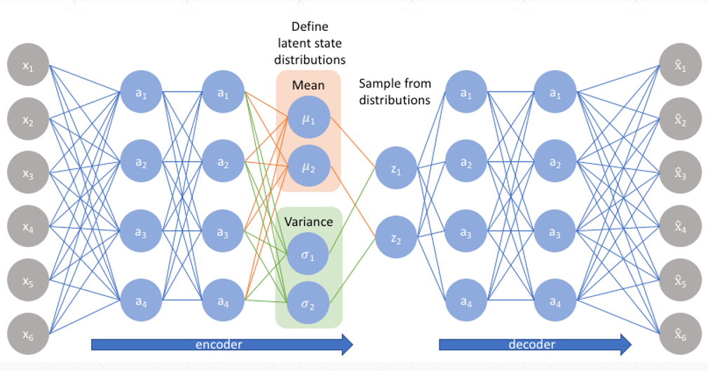
2、Variational Auto-Encoder
h_dim一半是均值(小网络),一半是方差(小网络),解码器从h层进行采样。
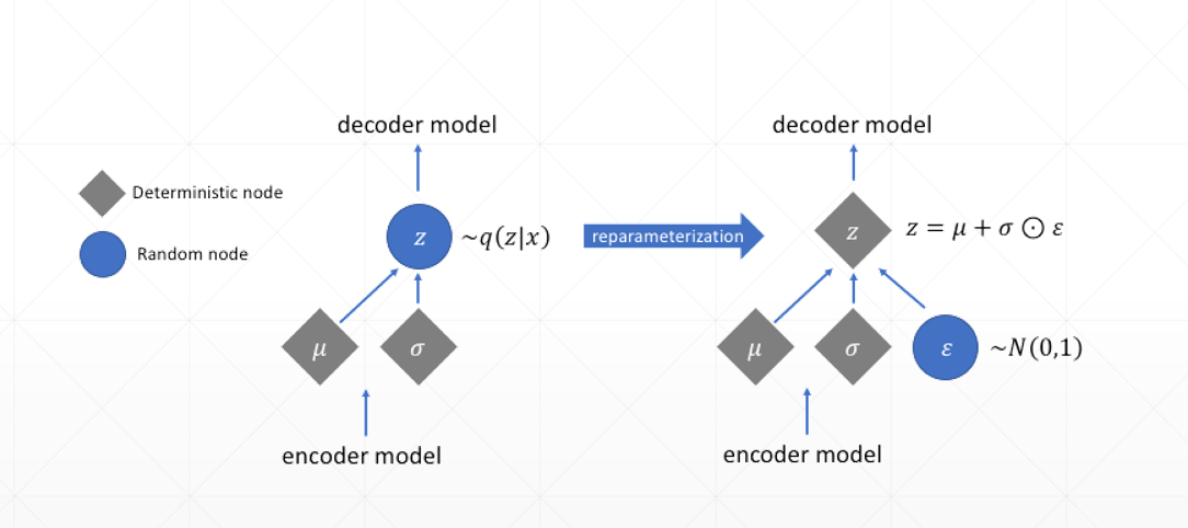
从均值和方差进行sample采样时,loss对均值和方差是不可导的,所以将原来的均值和方差的分布变成均值加方差的分布。
  1 import  os
  2 import  tensorflow as tf
  3 import  numpy as np
  4 from    tensorflow import keras
  5 from    tensorflow.keras import Sequential, layers
  6 from    PIL import Image
  7 from    matplotlib import pyplot as plt
  8
  9
 10 tf.random.set_seed(22)
 11 np.random.seed(22)
 12 os.environ['TF_CPP_MIN_LOG_LEVEL'] = '2'
 13 assert tf.__version__.startswith('2.')
 14
 15
 16 def save_images(imgs, name):
 17     new_im = Image.new('L', (280, 280))
 18
 19     index = 0
 20     for i in range(0, 280, 28):
 21         for j in range(0, 280, 28):
 22             im = imgs[index]
 23             im = Image.fromarray(im, mode='L')
 24             new_im.paste(im, (i, j))
 25             index += 1
 26
 27     new_im.save(name)
 28
 29
 30 h_dim = 20
 31 batchsz = 512
 32 lr = 1e-3
 33
 34
 35 (x_train, y_train), (x_test, y_test) = keras.datasets.fashion_mnist.load_data()
 36 x_train, x_test = x_train.astype(np.float32) / 255., x_test.astype(np.float32) / 255.
 37 # we do not need label
 38 train_db = tf.data.Dataset.from_tensor_slices(x_train)
 39 train_db = train_db.shuffle(batchsz * 5).batch(batchsz)
 40 test_db = tf.data.Dataset.from_tensor_slices(x_test)
 41 test_db = test_db.batch(batchsz)
 42
 43 print(x_train.shape, y_train.shape)
 44 print(x_test.shape, y_test.shape)
 45
 46 z_dim = 10
 47
 48 class VAE(keras.Model):
 49
 50     def __init__(self): #创建网络层
 51         super(VAE, self).__init__() # 输入为784
 52
 53         # Encoder h_dim可以分为均值网络和方差方差
 54         self.fc1 = layers.Dense(128)  #h_dim的上一层
 55         self.fc2 = layers.Dense(z_dim) # get mean prediction 分支结构,两个网络,得到均值  fc1->fc2
 56         self.fc3 = layers.Dense(z_dim) # 得到方差 fc1->fc3
 57
 58         # Decoder
 59         self.fc4 = layers.Dense(128)
 60         self.fc5 = layers.Dense(784)  #最后一层为784
 61
 62     def encoder(self, x):
 63
 64         h = tf.nn.relu(self.fc1(x))
 65         # get mean
 66         mu = self.fc2(h)
 67         # get variance
 68         log_var = self.fc3(h)  #log方差,正无穷到负无穷
 69
 70         return mu, log_var
 71
 72     def decoder(self, z):
 73
 74         out = tf.nn.relu(self.fc4(z))
 75         out = self.fc5(out)
 76
 77         return out
 78
 79     def reparameterize(self, mu, log_var):  #从均值和方差进行sample采样时,loss对均值和方差是不可导的,所以将原来的均值和方差的分布变成均值加方差的分布。
 80
 81         eps = tf.random.normal(log_var.shape)
 82
 83         std = tf.exp(log_var*0.5)
 84
 85         z = mu + std * eps
 86         return z
 87
 88     def call(self, inputs, training=None): # 网络层进行前向传播的过程
 89
 90         # [b, 784] => [b, z_dim], [b, z_dim] ,得到均值和方差的两个网络的logits
 91         mu, log_var = self.encoder(inputs)
 92         # reparameterization trick
 93         z = self.reparameterize(mu, log_var)
 94
 95         x_hat = self.decoder(z)
 96
 97         return x_hat, mu, log_var
 98
 99
100 model = VAE()
101 model.build(input_shape=(4, 784))
102 optimizer = tf.optimizers.Adam(lr)
103
104 for epoch in range(1000):
105
106     for step, x in enumerate(train_db):
107
108         x = tf.reshape(x, [-1, 784])
109
110         with tf.GradientTape() as tape:
111             x_rec_logits, mu, log_var = model(x)
112
113             rec_loss = tf.nn.sigmoid_cross_entropy_with_logits(labels=x, logits=x_rec_logits)
114             rec_loss = tf.reduce_sum(rec_loss) / x.shape[0]
115
116             # compute kl divergence (mu, var) ~ N (0, 1)  计算KL散度 假设为正态分布
117             # https://stats.stackexchange.com/questions/7440/kl-divergence-between-two-univariate-gaussians
118             # KL(p,q)=logσ2σ1+σ21+(μ1−μ2)22σ22−12
119
120             kl_div = -0.5 * (log_var + 1 - mu**2 - tf.exp(log_var)) #两个正态分布的KL散度的计算
121             kl_div = tf.reduce_sum(kl_div) / x.shape[0]  #求平均
122
123             loss = rec_loss + 1. * kl_div  #重建误差加KL误差
124
125         grads = tape.gradient(loss, model.trainable_variables) #计算梯度
126         optimizer.apply_gradients(zip(grads, model.trainable_variables))
127
128
129         if step % 100 == 0:
130             print(epoch, step, 'kl div:', float(kl_div), 'rec loss:', float(rec_loss))
131
132
133     # evaluation
134     z = tf.random.normal((batchsz, z_dim))
135     logits = model.decoder(z)  #随机给一个向量,因为解码器已经学习到了各个特征的分布,所以直接可以对新的图片进行生成
136     x_hat = tf.sigmoid(logits)  #结果进行sigmod
137     x_hat = tf.reshape(x_hat, [-1, 28, 28]).numpy() *255.  #还原到0-255
138     x_hat = x_hat.astype(np.uint8)
139     save_images(x_hat, 'vae_images/sampled_epoch%d.png'%epoch)
140
141     x = next(iter(test_db))
142     x = tf.reshape(x, [-1, 784])
143     x_hat_logits, _, _ = model(x)
144     x_hat = tf.sigmoid(x_hat_logits)
145     x_hat = tf.reshape(x_hat, [-1, 28, 28]).numpy() *255.
146     x_hat = x_hat.astype(np.uint8)
147     save_images(x_hat, 'vae_images/rec_epoch%d.png'%epoch)