吴恩达机器学习¶

编程作业1：单变量线性回归

该文章的实现步骤基本上是按照Cowry5的这篇文章：https://blog.csdn.net/Cowry5/article/details/83302646 中的线性回归章节来实现的，其中有略微改动。

编程语言：python 3.6

环境：jupyter notebook

 
      import numpy as np
import pandas as pd 
import matplotlib.pyplot as plt

path = 'ex1data1.txt'
# names添加列名，header用指定的行来作为标题，若原来无标题则设为none
data = pd.read_csv(path,names=['Population','Profit'])
data.head() 
     

	Population	Profit
0	6.1101	17.5920
1	5.5277	9.1302
2	8.5186	13.6620
3	7.0032	11.8540
4	5.8598	6.8233

data.describe() # 输出一些数据的统计量

	Population	Profit
count	97.000000	97.000000
mean	8.159800	5.839135
std	3.869884	5.510262
min	5.026900	-2.680700
25%	5.707700	1.986900
50%	6.589400	4.562300
75%	8.578100	7.046700
max	22.203000	24.147000

在开始任何任务之前，通过可视化来理解数据通常是有用的。对于这个数据集，你可以使用散点图来可视化数据，因为它只有两个属性（利润，人口）。（你在生活中遇到的许多其他问题都是多维度的，不能在二维图上画出来。）

 
      data.plot(kind='scatter', x='Population', y='Profit', figsize=(8,5))
plt.show(1)

现在让我们使用梯度下降来实现线性回归，以最小化cost function。首先，我们创建一个以 $θ$

其中，Hypothesis为：

当然，在该题情况中Hypothesis为：

我们把

x_{0}

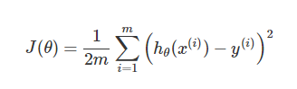
# 计算代价函数J（θ）
# 传入的X，y，t_theta都是列向量
# X 中的每行为x1,x2,x3.....
def compute_cost(X,y,theta):
    #print(t_theta.shape)
    inner = np.power(((X.dot(theta.T))-y),2) # 后面的2表示2次幂
    return sum(inner)/(2*len(X))
# 在训练集中插入一列1，方便计算
data.insert(0, 'Ones', 1)
# set X(training set), y(target variable)
# 设置训练集X，和目标变量y的值
cols = data.shape[1] # 获取列数
X = data.iloc[:,0:cols-1] # 输入向量X为前cols-1列
y = data.iloc[:,cols-1:cols] # 目标变量y为最后一列
#print(type(X))
#print(y)
X = np.array(X.values)
y = np.array(y.values)
theta = np.array([0,0]).reshape(1,2)
print(theta.shape)
print(X.shape)
print(y.shape)

(1, 2)
(97, 2)
(97, 1)

 
      parameters = int(theta.flatten().shape[0]) # 参数的数量
def gradientDescent(X, y, theta, alpha, epoch=1000):
    '''return theta, cost'''
    temp = np.array(np.zeros(theta.shape)) # 初始化一个theta临时矩阵
    parameters = int(theta.flatten().shape[0]) # 参数theta的数量
    cost = np.zeros(epoch) # 初始化一个ndarray，包含每次迭代后的cost
    m = X.shape[0] # 样本数量m
    
    for i in range(epoch):
        # 利用向量化同步计算theta值
        # 注意theta是一个行向量
        temp = theta - (alpha/m) * (X.dot(theta.T)- y).T.dot(X) # 得出一个theta行向量
        theta = temp
        cost[i] = compute_cost(X, y, theta) # 这个函数中，theta是变量，X，y是已知量
    return theta,cost # 迭代结束之后返回theta和cost值 
     

初始化学习速率和迭代次数：

alpha = 0.01
epoch = 2000

扫描二维码关注公众号，回复： 5927791 查看本文章

运行梯度下降算法，得出theta和cost：

final_theta, cost = gradientDescent(X, y, theta, alpha, epoch)

接下来我们可以使用计算出来的final_theta来计算训练模型的代价函数（计算误差）：

 
      final_cost = compute_cost(X, y, final_theta)
print(final_cost)
 
#[4.47802761]
population = np.linspace(data.Population.min(), data.Population.max(), 97)
population.shape 
     

(97,)

然后根据得出的参数theta，代入假设函数，绘制假设函数和训练数据的图像，直观的观测拟合程度：

 
      population = np.linspace(data.Population.min(), data.Population.max(), 100) # 横坐标
profit = final_theta[0,0] + (final_theta[0,1] * population) # 纵坐标，利润

fig, ax = plt.subplots(figsize=(8, 6))
ax.plot(population, profit, 'r', label='Prediction')
ax.scatter(data['Population'], data['Profit'], label='Training data')
ax.legend(loc=4) # 4表示标签在右下角
ax.set_xlabel('Population')
ax.set_ylabel('Profit')
ax.set_title('Prediction Profit by. Population Size')
plt.show() 
     

由于梯度下降过程中每一次迭代都会得到一个cost值，下面我们根据cost的值来绘制图像。我们通常使用绘制cost图像的方式来观测梯度下降算法是否正常的运行，若是算法运行正常，该图像会一直下降。

 
      fig,ax = plt.subplots(figsize=(8, 6))
ax.plot(np.arange(epoch), cost, 'r')
ax.set_xlabel('Iteration')
ax.set_ylabel('Cost')
ax.set_title('Error vs. Traning Epoch')
plt.show() 
     

可以由图像观察得出梯度下降算法运行正确，cost值是不断收敛的。
到此，第一次编程作业结束。

这次编程作业花了我很长时间才完成，归根到底是不熟悉矩阵运算造成的。理解和推导矩阵的运算花费了我一个小时的时间。
做完编程作业之后，我对线性回归和梯度下降算法有了更深入的了解，但是仍旧有很多疑惑，比如为什么这个算法是有用的，梯度下降算法是怎么得出的等等。
我打算先把吴恩达的课程看完，作业做完，对整个machine learning有一个总体的了解之后，再认真学习一遍林轩田的机器学习基石与机器学习技法，从整个理论上去了解机器学习。

吴恩达机器学习：编程作业1-单变量线性回归（Python实现）

吴恩达机器学习¶

编程作业1：单变量线性回归

猜你喜欢