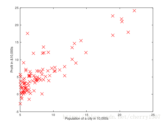
function plotData(x, y)
		figure;
		data = load('ex1data1.txt');
		x = data(:,1);
		y = data(:,2);
		plot(x,y,'rx','MarkerSize',10);
		xlabel('Population of a city in 10,000s');
		ylabel('Profit in &10,000s');
end
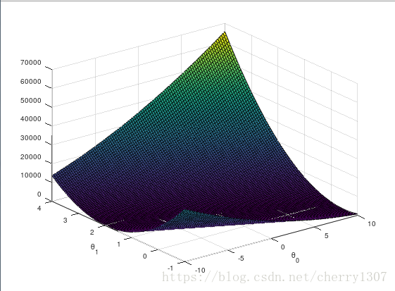
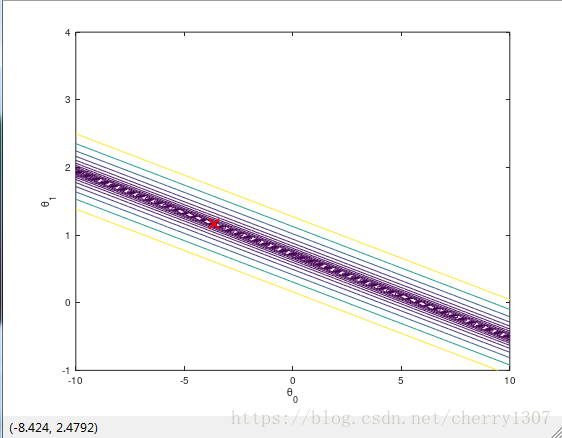
代价函数
%代价函数
%computeCost.m
function J = computeCost(X, y, theta)
		m = length(y);
		J = 0;
		h = X*theta;
		J = sum(h-y).^2/(2*m);
end
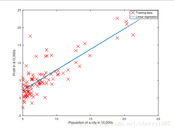
梯度下降法
%梯度下降
function [theta, J_history] = gradientDescent(X, y, theta, alpha, num_iters)
			m = length(y);
			J_history = zeros(num_iters, 1);
			for iter = 1:num_iters
				h=X*theta;
				t1 = theta(1) - alpha*(1/m)*sum(h-y);
				t2 = theta(2) - alpha*(1/m)*sum((h-y).*X(:,2));
				theta = [t1;t2];
		    J_history(iter) = computeCostMulti(X, y, theta);
end
end