转至:https://blog.csdn.net/bxg1065283526/article/details/80210359
最终文件看最后附录
Optimization Methods
Until now, you’ve always used Gradient Descent to update the parameters and minimize the cost. In this notebook, you will learn more advanced optimization methods that can speed up learning and perhaps even get you to a better final value for the cost function. Having a good optimization algorithm can be the difference between waiting days vs. just a few hours to get a good result. (到目前为止,您一直使用梯度下降来更新参数并将成本降至最低。在这款笔记本中,您将学习更先进的优化方法,可以加快学习速度,甚至可以让您获得更好的成本函数最终价值。有一个好的优化算法可以是等待几天之间的差异,只是几个小时才能得到一个好的结果)
Gradient descent goes “downhill” on a cost function J. Think of it as trying to do this:
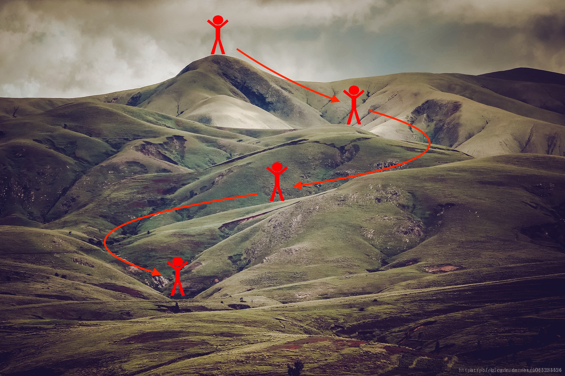
At each step of the training, you update your parameters following a certain direction to try to get to the lowest possible point

To get started, run the following code to import the libraries you will need.
import numpy as np
import matplotlib.pyplot as plt
import scipy.io
import math
import sklearn
import sklearn.datasets

from opt_utils import load_params_and_grads, initialize_parameters, forward_propagation, backward_propagation
from opt_utils import compute_cost, predict, predict_dec, plot_decision_boundary, load_dataset
from testCases import *

plt.rcParams['figure.figsize'] = (7.0, 4.0) # set default size of plots
plt.rcParams['image.interpolation'] = 'nearest'
plt.rcParams['image.cmap'] = 'gray'
其中testCases代码如下:
# -*- coding: utf-8 -*-

import numpy as np

def update_parameters_with_gd_test_case():
    np.random.seed(1)
    learning_rate = 0.01
    W1 = np.random.randn(2,3)
    b1 = np.random.randn(2,1)
    W2 = np.random.randn(3,3)
    b2 = np.random.randn(3,1)

    dW1 = np.random.randn(2,3)
    db1 = np.random.randn(2,1)
    dW2 = np.random.randn(3,3)
    db2 = np.random.randn(3,1)

    parameters = {"W1": W1, "b1": b1, "W2": W2, "b2": b2}
    grads = {"dW1": dW1, "db1": db1, "dW2": dW2, "db2": db2}

    return parameters, grads, learning_rate

"""
def update_parameters_with_sgd_checker(function, inputs, outputs):
    if function(inputs) == outputs:
        print("Correct")
    else:
        print("Incorrect")
"""

def random_mini_batches_test_case():
    np.random.seed(1)
    mini_batch_size = 64
    X = np.random.randn(12288, 148)
    Y = np.random.randn(1, 148) < 0.5
    return X, Y, mini_batch_size

def initialize_velocity_test_case():
    np.random.seed(1)
    W1 = np.random.randn(2,3)
    b1 = np.random.randn(2,1)
    W2 = np.random.randn(3,3)
    b2 = np.random.randn(3,1)
    parameters = {"W1": W1, "b1": b1, "W2": W2, "b2": b2}
    return parameters

def update_parameters_with_momentum_test_case():
    np.random.seed(1)
    W1 = np.random.randn(2,3)
    b1 = np.random.randn(2,1)
    W2 = np.random.randn(3,3)
    b2 = np.random.randn(3,1)

    dW1 = np.random.randn(2,3)
    db1 = np.random.randn(2,1)
    dW2 = np.random.randn(3,3)
    db2 = np.random.randn(3,1)
    parameters = {"W1": W1, "b1": b1, "W2": W2, "b2": b2}
    grads = {"dW1": dW1, "db1": db1, "dW2": dW2, "db2": db2}
    v = {'dW1': np.array([[ 0.,  0.,  0.],
        [ 0.,  0.,  0.]]), 'dW2': np.array([[ 0.,  0.,  0.],
        [ 0.,  0.,  0.],
        [ 0.,  0.,  0.]]), 'db1': np.array([[ 0.],
        [ 0.]]), 'db2': np.array([[ 0.],
        [ 0.],
        [ 0.]])}
    return parameters, grads, v

def initialize_adam_test_case():
    np.random.seed(1)
    W1 = np.random.randn(2,3)
    b1 = np.random.randn(2,1)
    W2 = np.random.randn(3,3)
    b2 = np.random.randn(3,1)
    parameters = {"W1": W1, "b1": b1, "W2": W2, "b2": b2}
    return parameters

def update_parameters_with_adam_test_case():
    np.random.seed(1)
    v, s = ({'dW1': np.array([[ 0.,  0.,  0.],
         [ 0.,  0.,  0.]]), 'dW2': np.array([[ 0.,  0.,  0.],
         [ 0.,  0.,  0.],
         [ 0.,  0.,  0.]]), 'db1': np.array([[ 0.],
         [ 0.]]), 'db2': np.array([[ 0.],
         [ 0.],
         [ 0.]])}, {'dW1': np.array([[ 0.,  0.,  0.],
         [ 0.,  0.,  0.]]), 'dW2': np.array([[ 0.,  0.,  0.],
         [ 0.,  0.,  0.],
         [ 0.,  0.,  0.]]), 'db1': np.array([[ 0.],
         [ 0.]]), 'db2': np.array([[ 0.],
         [ 0.],
         [ 0.]])})
    W1 = np.random.randn(2,3)
    b1 = np.random.randn(2,1)
    W2 = np.random.randn(3,3)
    b2 = np.random.randn(3,1)

    dW1 = np.random.randn(2,3)
    db1 = np.random.randn(2,1)
    dW2 = np.random.randn(3,3)
    db2 = np.random.randn(3,1)

    parameters = {"W1": W1, "b1": b1, "W2": W2, "b2": b2}
    grads = {"dW1": dW1, "db1": db1, "dW2": dW2, "db2": db2}

    return parameters, grads, v, s
opt_utils代码如下:
# -*- coding: utf-8 -*-

import numpy as np
import matplotlib.pyplot as plt
import sklearn
import sklearn.datasets

def sigmoid(x):
    """
    Compute the sigmoid of x

    Arguments:
    x -- A scalar or numpy array of any size.

    Return:
    s -- sigmoid(x)
    """
    s = 1/(1+np.exp(-x))
    return s

def relu(x):
    """
    Compute the relu of x

    Arguments:
    x -- A scalar or numpy array of any size.

    Return:
    s -- relu(x)
    """
    s = np.maximum(0,x)

    return s


def load_params_and_grads(seed=1):
    np.random.seed(seed)
    W1 = np.random.randn(2,3)
    b1 = np.random.randn(2,1)
    W2 = np.random.randn(3,3)
    b2 = np.random.randn(3,1)

    dW1 = np.random.randn(2,3)
    db1 = np.random.randn(2,1)
    dW2 = np.random.randn(3,3)
    db2 = np.random.randn(3,1)

    return W1, b1, W2, b2, dW1, db1, dW2, db2

def initialize_parameters(layer_dims):
    """
    Arguments:
    layer_dims -- python array (list) containing the dimensions of each layer in our network

    Returns:
    parameters -- python dictionary containing your parameters "W1", "b1", ..., "WL", "bL":
                    W1 -- weight matrix of shape (layer_dims[l], layer_dims[l-1])
                    b1 -- bias vector of shape (layer_dims[l], 1)
                    Wl -- weight matrix of shape (layer_dims[l-1], layer_dims[l])
                    bl -- bias vector of shape (1, layer_dims[l])

    Tips:
    - For example: the layer_dims for the "Planar Data classification model" would have been [2,2,1].
    This means W1's shape was (2,2), b1 was (1,2), W2 was (2,1) and b2 was (1,1). Now you have to generalize it!
    - In the for loop, use parameters['W' + str(l)] to access Wl, where l is the iterative integer.
    """

    np.random.seed(3)
    parameters = {}
    L = len(layer_dims) # number of layers in the network

    for l in range(1, L):
        parameters['W' + str(l)] = np.random.randn(layer_dims[l], layer_dims[l-1])*  np.sqrt(2 / layer_dims[l-1])
        parameters['b' + str(l)] = np.zeros((layer_dims[l], 1))

        assert(parameters['W' + str(l)].shape == layer_dims[l], layer_dims[l-1])
        assert(parameters['W' + str(l)].shape == layer_dims[l], 1)

    return parameters

def forward_propagation(X, parameters):
    """
    Implements the forward propagation (and computes the loss) presented in Figure 2.

    Arguments:
    X -- input dataset, of shape (input size, number of examples)
    parameters -- python dictionary containing your parameters "W1", "b1", "W2", "b2", "W3", "b3":
                    W1 -- weight matrix of shape ()
                    b1 -- bias vector of shape ()
                    W2 -- weight matrix of shape ()
                    b2 -- bias vector of shape ()
                    W3 -- weight matrix of shape ()
                    b3 -- bias vector of shape ()

    Returns:
    loss -- the loss function (vanilla logistic loss)
    """

    # retrieve parameters
    W1 = parameters["W1"]
    b1 = parameters["b1"]
    W2 = parameters["W2"]
    b2 = parameters["b2"]
    W3 = parameters["W3"]
    b3 = parameters["b3"]

    # LINEAR -> RELU -> LINEAR -> RELU -> LINEAR -> SIGMOID
    z1 = np.dot(W1, X) + b1
    a1 = relu(z1)
    z2 = np.dot(W2, a1) + b2
    a2 = relu(z2)
    z3 = np.dot(W3, a2) + b3
    a3 = sigmoid(z3)

    cache = (z1, a1, W1, b1, z2, a2, W2, b2, z3, a3, W3, b3)

    return a3, cache

def backward_propagation(X, Y, cache):
    """
    Implement the backward propagation presented in figure 2.

    Arguments:
    X -- input dataset, of shape (input size, number of examples)
    Y -- true "label" vector (containing 0 if cat, 1 if non-cat)
    cache -- cache output from forward_propagation()

    Returns:
    gradients -- A dictionary with the gradients with respect to each parameter, activation and pre-activation variables
    """
    m = X.shape[1]
    (z1, a1, W1, b1, z2, a2, W2, b2, z3, a3, W3, b3) = cache

    dz3 = 1./m * (a3 - Y)
    dW3 = np.dot(dz3, a2.T)
    db3 = np.sum(dz3, axis=1, keepdims = True)

    da2 = np.dot(W3.T, dz3)
    dz2 = np.multiply(da2, np.int64(a2 > 0))
    dW2 = np.dot(dz2, a1.T)
    db2 = np.sum(dz2, axis=1, keepdims = True)

    da1 = np.dot(W2.T, dz2)
    dz1 = np.multiply(da1, np.int64(a1 > 0))
    dW1 = np.dot(dz1, X.T)
    db1 = np.sum(dz1, axis=1, keepdims = True)

    gradients = {"dz3": dz3, "dW3": dW3, "db3": db3,
                 "da2": da2, "dz2": dz2, "dW2": dW2, "db2": db2,
                 "da1": da1, "dz1": dz1, "dW1": dW1, "db1": db1}

    return gradients

def compute_cost(a3, Y):

    """
    Implement the cost function

    Arguments:
    a3 -- post-activation, output of forward propagation
    Y -- "true" labels vector, same shape as a3

    Returns:
    cost - value of the cost function
    """
    m = Y.shape[1]

    logprobs = np.multiply(-np.log(a3),Y) + np.multiply(-np.log(1 - a3), 1 - Y)
    cost = 1./m * np.sum(logprobs)

    return cost

def predict(X, y, parameters):
    """
    This function is used to predict the results of a  n-layer neural network.

    Arguments:
    X -- data set of examples you would like to label
    parameters -- parameters of the trained model

    Returns:
    p -- predictions for the given dataset X
    """

    m = X.shape[1]
    p = np.zeros((1,m), dtype = np.int)

    # Forward propagation
    a3, caches = forward_propagation(X, parameters)

    # convert probas to 0/1 predictions
    for i in range(0, a3.shape[1]):
        if a3[0,i] > 0.5:
            p[0,i] = 1
        else:
            p[0,i] = 0

    # print results

    #print ("predictions: " + str(p[0,:]))
    #print ("true labels: " + str(y[0,:]))
    print("Accuracy: "  + str(np.mean((p[0,:] == y[0,:]))))

    return p

def predict_dec(parameters, X):
    """
    Used for plotting decision boundary.

    Arguments:
    parameters -- python dictionary containing your parameters
    X -- input data of size (m, K)

    Returns
    predictions -- vector of predictions of our model (red: 0 / blue: 1)
    """

    # Predict using forward propagation and a classification threshold of 0.5
    a3, cache = forward_propagation(X, parameters)
    predictions = (a3 > 0.5)
    return predictions

def plot_decision_boundary(model, X, y):
    # Set min and max values and give it some padding
    x_min, x_max = X[0, :].min() - 1, X[0, :].max() + 1
    y_min, y_max = X[1, :].min() - 1, X[1, :].max() + 1
    h = 0.01
    # Generate a grid of points with distance h between them
    xx, yy = np.meshgrid(np.arange(x_min, x_max, h), np.arange(y_min, y_max, h))
    # Predict the function value for the whole grid
    Z = model(np.c_[xx.ravel(), yy.ravel()])
    Z = Z.reshape(xx.shape)
    # Plot the contour and training examples
    plt.contourf(xx, yy, Z, cmap=plt.cm.Spectral)
    plt.ylabel('x2')
    plt.xlabel('x1')
    plt.scatter(X[0, :], X[1, :], c=y, cmap=plt.cm.Spectral)
    plt.show()

def load_dataset(is_plot = True):
    np.random.seed(3)
    train_X, train_Y = sklearn.datasets.make_moons(n_samples=300, noise=.2) #300 #0.2
    # Visualize the data
    if is_plot:
        plt.scatter(train_X[:, 0], train_X[:, 1], c=train_Y, s=40, cmap=plt.cm.Spectral);
    train_X = train_X.T
    train_Y = train_Y.reshape((1, train_Y.shape[0]))

    return train_X, train_Y
1 - Gradient Descent
A simple optimization method in machine learning is gradient descent (GD). When you take gradient steps with respect to all m examples on each step, it is also called Batch Gradient Descent. (机器学习中一个简单的优化方法是梯度下降(GD)。当您对每个步骤的所有m示例采取渐变步骤时,它也被称为批处理渐变下降(Batch Gradient Descent))
Warm-up exercise: Implement the gradient descent update rule. The gradient descent rule is, for l=1,...,L:
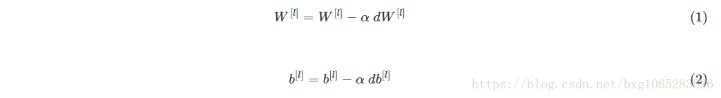
where L is the number of layers and α is the learning rate. All parameters should be stored in the parameters dictionary. Note that the iterator l starts at 0 in the for loop while the first parameters are W[1] and b[1]. You need to shift l to l+1when coding.(其中L是层数,α是学习率。所有的参数都应该存储在parameters字典中。请注意,迭代器l在for循环中从0开始,而第一个参数是W[1]和b[1]
。编码时需要将l移到l + 1。)
def update_parameters_with_gd(parameters, grads, learning_rate):
    """
    Update parameters using one step of gradient descent

    Arguments:
    parameters -- python dictionary containing your parameters to be updated:
                    parameters['W' + str(l)] = Wl
                    parameters['b' + str(l)] = bl
    grads -- python dictionary containing your gradients to update each parameters:
                    grads['dW' + str(l)] = dWl
                    grads['db' + str(l)] = dbl
    learning_rate -- the learning rate, scalar.

    Returns:
    parameters -- python dictionary containing your updated parameters
    """

    L = len(parameters) // 2 # number of layers in the neural networks

    # Update rule for each parameter
    for l in range(L):
        ### START CODE HERE ### (approx. 2 lines)
        parameters["W" + str(l+1)] = parameters["W" + str(l+1)] - learning_rate*grads["dW" + str(l+1)]
        parameters["b" + str(l+1)] = parameters["b" + str(l+1)] -learning_rate*grads["db" + str(l+1)]
        ### END CODE HERE ###

    return parameters
parameters, grads, learning_rate = update_parameters_with_gd_test_case()

parameters = update_parameters_with_gd(parameters, grads, learning_rate)
print("W1 = " + str(parameters["W1"]))
print("b1 = " + str(parameters["b1"]))
print("W2 = " + str(parameters["W2"]))
print("b2 = " + str(parameters["b2"]))
运行结果:
W1 = [[ 1.63535156 -0.62320365 -0.53718766]
 [-1.07799357  0.85639907 -2.29470142]]
b1 = [[ 1.74604067]
 [-0.75184921]]
W2 = [[ 0.32171798 -0.25467393  1.46902454]
 [-2.05617317 -0.31554548 -0.3756023 ]
 [ 1.1404819  -1.09976462 -0.1612551 ]]
b2 = [[-0.88020257]
 [ 0.02561572]
 [ 0.57539477]]
A variant of this is Stochastic Gradient Descent (SGD), which is equivalent to mini-batch gradient descent where each mini-batch has just 1 example. The update rule that you have just implemented does not change. What changes is that you would be computing gradients on just one training example at a time, rather than on the whole training set. The code examples below illustrate the difference between stochastic gradient descent and (batch) gradient descent. (这是一个随机梯度下降(SGD),相当于小批量梯度下降,每个小批量只有1个例子。您刚刚实施的更新规则不会更改。什么样的变化是你一次只能在一个训练样例上计算梯度,而不是在整个训练集上。下面的代码示例说明了随机梯度下降和(批量)梯度下降之间的差异)
- (Batch) Gradient Descent:
A variant of this is Stochastic Gradient Descent (SGD), which is equivalent to mini-batch gradient descent where each mini-batch has just 1 example. The update rule that you have just implemented does not change. What changes is that you would be computing gradients on just one training example at a time, rather than on the whole training set. The code examples below illustrate the difference between stochastic gradient descent and (batch) gradient descent. (这是一个随机梯度下降(SGD),相当于小批量梯度下降,每个小批量只有1个例子。您刚刚实施的更新规则不会更改。什么样的变化是你一次只能在一个训练样例上计算梯度,而不是在整个训练集上。下面的代码示例说明了随机梯度下降和(批量)梯度下降之间的差异)
X = data_input
Y = labels
parameters = initialize_parameters(layers_dims)
for i in range(0, num_iterations):
    # Forward propagation
    a, caches = forward_propagation(X, parameters)
    # Compute cost.
    cost = compute_cost(a, Y)
    # Backward propagation.
    grads = backward_propagation(a, caches, parameters)
    # Update parameters.
    parameters = update_parameters(parameters, grads)
- Stochastic Gradient Descent:
X = data_input
Y = labels
parameters = initialize_parameters(layers_dims)
for i in range(0, num_iterations):
    for j in range(0, m):
        # Forward propagation
        a, caches = forward_propagation(X[:,j], parameters)
        # Compute cost
        cost = compute_cost(a, Y[:,j])
        # Backward propagation
        grads = backward_propagation(a, caches, parameters)
        # Update parameters.
        parameters = update_parameters(parameters, grads)
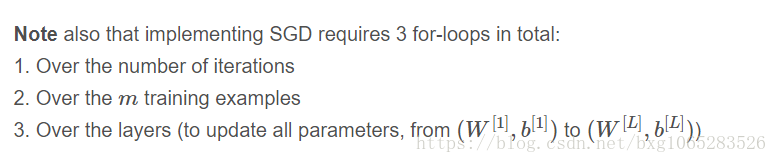
In Stochastic Gradient Descent, you use only 1 training example before updating the gradients. When the training set is large, SGD can be faster. But the parameters will “oscillate” toward the minimum rather than converge smoothly. Here is an illustration of this(在随机梯度下降中,在更新梯度之前,只使用1个训练样例。当训练集大时,SGD可以更快。但是这些参数会向最小值“摆动”而不是平稳地收敛。这是一个例子):

Figure 1 : SGD vs GD
“+” denotes a minimum of the cost. SGD leads to many oscillations to reach convergence. But each step is a lot faster to compute for SGD than for GD, as it uses only one training example (vs. the whole batch for GD).
In practice, you’ll often get faster results if you do not use neither the whole training set, nor only one training example, to perform each update. Mini-batch gradient descent uses an intermediate number of examples for each step. With mini-batch gradient descent, you loop over the mini-batches instead of looping over individual training examples(在实践中,如果您不使用整个训练集,也不仅仅是一个训练样例来执行每个更新,您通常会得到更快的结果。小批量梯度下降为每个步骤使用中间数量的示例。通过小批量梯度下降,可以循环使用小批量,而不是循环遍历各个训练示例).
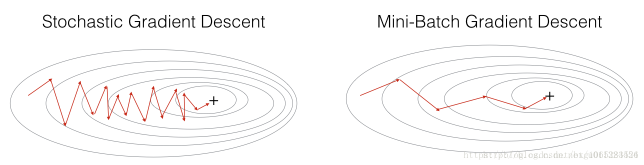
Figure 2 : SGD vs Mini-Batch GD
“+” denotes a minimum of the cost. Using mini-batches in your optimization algorithm often leads to faster optimization.
What you should remember:
- The difference between gradient descent, mini-batch gradient descent and stochastic gradient descent is the number of examples you use to perform one update step(在梯度下降,小批量梯度下降和随机梯度下降之间的差异是用于执行一个更新步骤的示例数量).
- You have to tune a learning rate hyperparameter α(你必须调整学习速率超参数α).
- With a well-turned mini-batch size, usually it outperforms either gradient descent or stochastic gradient descent (particularly when the training set is large)(在小批量生产的情况下,通常它的性能优于梯度下降或随机梯度下降(特别是当训练集较大时)).
2 - Mini-Batch Gradient descent
Let’s learn how to build mini-batches from the training set (X, Y).
There are two steps:
- Shuffle: Create a shuffled version of the training set (X, Y) as shown below. Each column of X and Y represents a training example. Note that the random shuffling is done synchronously between X and Y. Such that after the shuffling the ithcolumn of X is the example corresponding to the ith label in Y. The shuffling step ensures that examples will be split randomly into different mini-batches. (创建训练集(X,Y)的混洗版本,如下所示。 X和Y的每一列代表一个训练样例。注意随机混洗是在X和Y之间同步完成的。这样,在混洗之后,X的ith列是对应于Y中的ith标签的例子。混洗步骤确保那个例子将被随机分成不同的小批量)

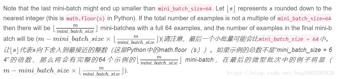
- Partition: Partition the shuffled (X, Y) into mini-batches of size
mini_batch_size(here 64). Note that the number of training examples is not always divisible bymini_batch_size. The last mini batch might be smaller, but you don’t need to worry about this. When the final mini-batch is smaller than the fullmini_batch_size, it will look like this(将混洗的(X,Y)划分为大小为mini_batch_size的小批量(这里是64)。请注意,训练示例的数量并不总是可以被mini_batch_size整除。最后一个小批量可能会更小,但您不必担心这一点。当最后一个小批量比完整的mini_batch_size小时,看起来就像这样):

Exercise: Implement random_mini_batches. We coded the shuffling part for you. To help you with the partitioning step, we give you the following code that selects the indexes for the 1st and 2nd mini-batches(实现random_mini_batches。我们为你编码洗牌部分。为了帮助您进行分区步骤,我们为您提供以下代码,用于选择1st和2nd小批量的索引):
first_mini_batch_X = shuffled_X[:, 0 : mini_batch_size]
second_mini_batch_X = shuffled_X[:, mini_batch_size : 2 * mini_batch_size]
...
def random_mini_batches(X, Y, mini_batch_size = 64, seed = 0):
    """
    Creates a list of random minibatches from (X, Y)

    Arguments:
    X -- input data, of shape (input size, number of examples)
    Y -- true "label" vector (1 for blue dot / 0 for red dot), of shape (1, number of examples)
    mini_batch_size -- size of the mini-batches, integer

    Returns:
    mini_batches -- list of synchronous (mini_batch_X, mini_batch_Y)
    """

    np.random.seed(seed)            # To make your "random" minibatches the same as ours
    m = X.shape[1]                  # number of training examples
    mini_batches = []

    # Step 1: Shuffle (X, Y)
    permutation = list(np.random.permutation(m))
    shuffled_X = X[:, permutation]
    shuffled_Y = Y[:, permutation].reshape((1,m))

    # Step 2: Partition (shuffled_X, shuffled_Y). Minus the end case.
    num_complete_minibatches = math.floor(m/mini_batch_size) # number of mini batches of size mini_batch_size in your partitionning
    for k in range(0, num_complete_minibatches):
        ### START CODE HERE ### (approx. 2 lines)
        mini_batch_X = shuffled_X[:,k * mini_batch_size : (k+1) * mini_batch_size]
        mini_batch_Y = shuffled_Y[:,k * mini_batch_size : (k+1) * mini_batch_size]
        ### END CODE HERE ###
        mini_batch = (mini_batch_X, mini_batch_Y)
        mini_batches.append(mini_batch)

    # Handling the end case (last mini-batch < mini_batch_size)
    if m % mini_batch_size != 0:
        ### START CODE HERE ### (approx. 2 lines)
        mini_batch_X = shuffled_X[:,num_complete_minibatches * mini_batch_size:]
        mini_batch_Y = shuffled_Y[:,num_complete_minibatches * mini_batch_size:]
        ### END CODE HERE ###
        mini_batch = (mini_batch_X, mini_batch_Y)
        mini_batches.append(mini_batch)

    return mini_batches
X_assess, Y_assess, mini_batch_size = random_mini_batches_test_case()
mini_batches = random_mini_batches(X_assess, Y_assess, mini_batch_size)

print ("shape of the 1st mini_batch_X: " + str(mini_batches[0][0].shape))
print ("shape of the 2nd mini_batch_X: " + str(mini_batches[1][0].shape))
print ("shape of the 3rd mini_batch_X: " + str(mini_batches[2][0].shape))
print ("shape of the 1st mini_batch_Y: " + str(mini_batches[0][1].shape))
print ("shape of the 2nd mini_batch_Y: " + str(mini_batches[1][1].shape))
print ("shape of the 3rd mini_batch_Y: " + str(mini_batches[2][1].shape))
print ("mini batch sanity check: " + str(mini_batches[0][0][0][0:3]))
运行结果:
shape of the 1st mini_batch_X: (12288, 64)
shape of the 2nd mini_batch_X: (12288, 64)
shape of the 3rd mini_batch_X: (12288, 64)
shape of the 1st mini_batch_Y: (1, 64)
shape of the 2nd mini_batch_Y: (1, 64)
shape of the 3rd mini_batch_Y: (1, 20)
mini batch sanity check: [ 0.90085595 -0.7612069   0.2344157 ]
What you should remember:
- Shuffling and Partitioning are the two steps required to build mini-batches(Shuffling和Partitioning是构建小批量所需的两个步骤)
- Powers of two are often chosen to be the mini-batch size, e.g., 16, 32, 64, 128.(通常选择2的幂的小批量,例如16,32,64,128)
3 - Momentum
Because mini-batch gradient descent makes a parameter update after seeing just a subset of examples, the direction of the update has some variance, and so the path taken by mini-batch gradient descent will “oscillate” toward convergence. Using momentum can reduce these oscillations. (由于小批量梯度下降在仅看到一个子集的例子之后进行参数更新,因此更新的方向有一定的变化,所以小批量梯度下降所采用的路径将会“趋于”收敛。使用动量可以减少这些振荡)
Momentum takes into account the past gradients to smooth out the update. We will store the ‘direction’ of the previous gradients in the variable v. Formally, this will be the exponentially weighted average of the gradient on previous steps. You can also think of v as the “velocity” of a ball rolling downhill, building up speed (and momentum) according to the direction of the gradient/slope of the hill. (动量考虑到过去的渐变来平滑更新。我们将把以前渐变的“方向”存储在变量v中。形式上,这将是前面步骤中梯度的指数加权平均值。你也可以把v想象成下坡滚动的“速度”,根据山坡/坡度的方向建立速度(和动量))
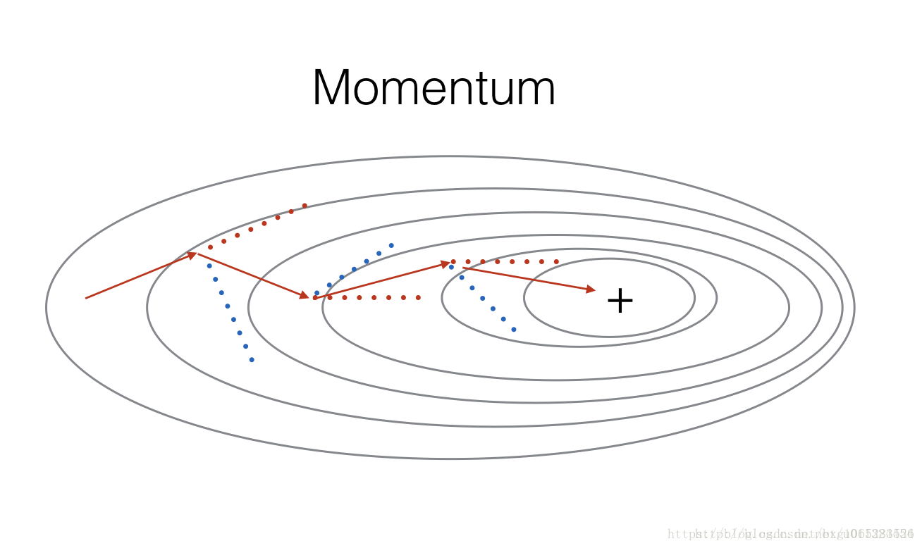
Figure 3: The red arrows shows the direction taken by one step of mini-batch gradient descent with momentum. The blue points show the direction of the gradient (with respect to the current mini-batch) on each step. Rather than just following the gradient, we let the gradient influence v and then take a step in the direction of v(红色的箭头显示了一步一步的小批量梯度下降的动力。蓝色的点显示每个步骤的梯度(相对于当前小批量)的方向。我们不是只跟随渐变,而是让渐变影响v,然后向v
的方向迈进一步).

v["dW" + str(l+1)] = ... #(numpy array of zeros with the same shape as parameters["W" + str(l+1)])
v["db" + str(l+1)] = ... #(numpy array of zeros with the same shape as parameters["b" + str(l+1)])
Note that the iterator l starts at 0 in the for loop while the first parameters are v[“dW1”] and v[“db1”] (that’s a “one” on the superscript). This is why we are shifting l to l+1 in the for loop.(迭代器l在for循环中从0开始,而第一个参数是v[“dW1”]和v[“db1”](这是上标中的“1”)。这就是为什么我们在l循环中将l移到l + 1的原因)
def initialize_velocity(parameters):
    """
    Initializes the velocity as a python dictionary with:
                - keys: "dW1", "db1", ..., "dWL", "dbL"
                - values: numpy arrays of zeros of the same shape as the corresponding gradients/parameters.
    Arguments:
    parameters -- python dictionary containing your parameters.
                    parameters['W' + str(l)] = Wl
                    parameters['b' + str(l)] = bl

    Returns:
    v -- python dictionary containing the current velocity.
                    v['dW' + str(l)] = velocity of dWl
                    v['db' + str(l)] = velocity of dbl
    """

    L = len(parameters) // 2 # number of layers in the neural networks
    v = {}

    # Initialize velocity
    for l in range(L):
        ### START CODE HERE ### (approx. 2 lines)
        v["dW" + str(l+1)] = np.zeros(parameters["W" + str(l+1)].shape)
        v["db" + str(l+1)] = np.zeros(parameters["b" + str(l+1)].shape)
        ### END CODE HERE ###

    return v
parameters = initialize_velocity_test_case()

v = initialize_velocity(parameters)
print("v[\"dW1\"] = " + str(v["dW1"]))
print("v[\"db1\"] = " + str(v["db1"]))
print("v[\"dW2\"] = " + str(v["dW2"]))
print("v[\"db2\"] = " + str(v["db2"]))
运行结果:
v["dW1"] = [[0. 0. 0.]
 [0. 0. 0.]]
v["db1"] = [[0.]
 [0.]]
v["dW2"] = [[0. 0. 0.]
 [0. 0. 0.]
 [0. 0. 0.]]
v["db2"] = [[0.]
 [0.]
 [0.]]

def update_parameters_with_momentum(parameters, grads, v, beta, learning_rate):
    """
    Update parameters using Momentum

    Arguments:
    parameters -- python dictionary containing your parameters:
                    parameters['W' + str(l)] = Wl
                    parameters['b' + str(l)] = bl
    grads -- python dictionary containing your gradients for each parameters:
                    grads['dW' + str(l)] = dWl
                    grads['db' + str(l)] = dbl
    v -- python dictionary containing the current velocity:
                    v['dW' + str(l)] = ...
                    v['db' + str(l)] = ...
    beta -- the momentum hyperparameter, scalar
    learning_rate -- the learning rate, scalar

    Returns:
    parameters -- python dictionary containing your updated parameters
    v -- python dictionary containing your updated velocities
    """

    L = len(parameters) // 2 # number of layers in the neural networks

    # Momentum update for each parameter
    for l in range(L):

        ### START CODE HERE ### (approx. 4 lines)
        # compute velocities
        v["dW" + str(l+1)] = np.dot(beta,v["dW"+str(l+1)]) + np.dot(1-beta,grads["dW"+str(l+1)])
        v["db" + str(l+1)] = np.dot(beta,v["db"+str(l+1)]) + np.dot(1-beta,grads["db"+str(l+1)])
        # update parameters
        parameters["W" + str(l+1)] = parameters["W" + str(l+1)] - learning_rate*v["dW" + str(l+1)]
        parameters["b" + str(l+1)] = parameters["b" + str(l+1)] - learning_rate*v["db" + str(l+1)]
        ### END CODE HERE ###

    return parameters, v
parameters, grads, v = update_parameters_with_momentum_test_case()

parameters, v = update_parameters_with_momentum(parameters, grads, v, beta = 0.9, learning_rate = 0.01)
print("W1 = " + str(parameters["W1"]))
print("b1 = " + str(parameters["b1"]))
print("W2 = " + str(parameters["W2"]))
print("b2 = " + str(parameters["b2"]))
print("v[\"dW1\"] = " + str(v["dW1"]))
print("v[\"db1\"] = " + str(v["db1"]))
print("v[\"dW2\"] = " + str(v["dW2"]))
print("v[\"db2\"] = " + str(v["db2"]))
运行结果:
W1 = [[ 1.62544598 -0.61290114 -0.52907334]
 [-1.07347112  0.86450677 -2.30085497]]
b1 = [[ 1.74493465]
 [-0.76027113]]
W2 = [[ 0.31930698 -0.24990073  1.4627996 ]
 [-2.05974396 -0.32173003 -0.38320915]
 [ 1.13444069 -1.0998786  -0.1713109 ]]
b2 = [[-0.87809283]
 [ 0.04055394]
 [ 0.58207317]]
v["dW1"] = [[-0.11006192  0.11447237  0.09015907]
 [ 0.05024943  0.09008559 -0.06837279]]
v["db1"] = [[-0.01228902]
 [-0.09357694]]
v["dW2"] = [[-0.02678881  0.05303555 -0.06916608]
 [-0.03967535 -0.06871727 -0.08452056]
 [-0.06712461 -0.00126646 -0.11173103]]
v["db2"] = [[0.02344157]
 [0.16598022]
 [0.07420442]]
What you should remember:
- Momentum takes past gradients into account to smooth out the steps of gradient descent. It can be applied with batch gradient descent, mini-batch gradient descent or stochastic gradient descent.(Momentum将渐变考虑在内以平滑梯度下降的步骤。可以采用分批梯度下降法,小批量梯度下降法或随机梯度下降法)
- You have to tune a momentum hyperparameter β and a learning rate α.(你必须调整动量超参数β和学习率α)
4 - Adam
Adam is one of the most effective optimization algorithms for training neural networks. It combines ideas from RMSProp (described in lecture) and Momentum. (Adam是训练神经网络最有效的优化算法之一。它结合了RMSProp(讲座中介绍)和Momentum的想法)

As usual, we will store all parameters in the parameters dictionary
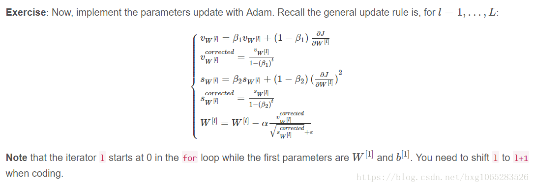
Exercise: Initialize the Adam variables v,s which keep track of the past information.
Instruction: The variables v,s are python dictionaries that need to be initialized with arrays of zeros. Their keys are the same as for grads, that is:
for l=1,...,L:
v["dW" + str(l+1)] = ... #(numpy array of zeros with the same shape as parameters["W" + str(l+1)])
v["db" + str(l+1)] = ... #(numpy array of zeros with the same shape as parameters["b" + str(l+1)])
s["dW" + str(l+1)] = ... #(numpy array of zeros with the same shape as parameters["W" + str(l+1)])
s["db" + str(l+1)] = ... #(numpy array of zeros with the same shape as parameters["b" + str(l+1)])
def initialize_adam(parameters) :
    """
    Initializes v and s as two python dictionaries with:
                - keys: "dW1", "db1", ..., "dWL", "dbL"
                - values: numpy arrays of zeros of the same shape as the corresponding gradients/parameters.

    Arguments:
    parameters -- python dictionary containing your parameters.
                    parameters["W" + str(l)] = Wl
                    parameters["b" + str(l)] = bl

    Returns:
    v -- python dictionary that will contain the exponentially weighted average of the gradient.
                    v["dW" + str(l)] = ...
                    v["db" + str(l)] = ...
    s -- python dictionary that will contain the exponentially weighted average of the squared gradient.
                    s["dW" + str(l)] = ...
                    s["db" + str(l)] = ...

    """

    L = len(parameters) // 2 # number of layers in the neural networks
    v = {}
    s = {}

    # Initialize v, s. Input: "parameters". Outputs: "v, s".
    for l in range(L):
    ### START CODE HERE ### (approx. 4 lines)
        v["dW" + str(l+1)] = np.zeros(parameters["W" + str(l+1)].shape)
        v["db" + str(l+1)] = np.zeros(parameters["b" + str(l+1)].shape)
        s["dW" + str(l+1)] = np.zeros(parameters["W" + str(l+1)].shape)
        s["db" + str(l+1)] = np.zeros(parameters["b" + str(l+1)].shape)
    ### END CODE HERE ###

    return v, s
parameters = initialize_adam_test_case()

v, s = initialize_adam(parameters)
print("v[\"dW1\"] = " + str(v["dW1"]))
print("v[\"db1\"] = " + str(v["db1"]))
print("v[\"dW2\"] = " + str(v["dW2"]))
print("v[\"db2\"] = " + str(v["db2"]))
print("s[\"dW1\"] = " + str(s["dW1"]))
print("s[\"db1\"] = " + str(s["db1"]))
print("s[\"dW2\"] = " + str(s["dW2"]))
print("s[\"db2\"] = " + str(s["db2"]))
运行结果:
v["dW1"] = [[0. 0. 0.]
 [0. 0. 0.]]
v["db1"] = [[0.]
 [0.]]
v["dW2"] = [[0. 0. 0.]
 [0. 0. 0.]
 [0. 0. 0.]]
v["db2"] = [[0.]
 [0.]
 [0.]]
s["dW1"] = [[0. 0. 0.]
 [0. 0. 0.]]
s["db1"] = [[0.]
 [0.]]
s["dW2"] = [[0. 0. 0.]
 [0. 0. 0.]
 [0. 0. 0.]]
s["db2"] = [[0.]
[0.]
 [0.]]
def update_parameters_with_adam(parameters, grads, v, s, t, learning_rate = 0.01,
                                beta1 = 0.9, beta2 = 0.999,  epsilon = 1e-8):
    """
    Update parameters using Adam

    Arguments:
    parameters -- python dictionary containing your parameters:
                    parameters['W' + str(l)] = Wl
                    parameters['b' + str(l)] = bl
    grads -- python dictionary containing your gradients for each parameters:
                    grads['dW' + str(l)] = dWl
                    grads['db' + str(l)] = dbl
    v -- Adam variable, moving average of the first gradient, python dictionary
    s -- Adam variable, moving average of the squared gradient, python dictionary
    learning_rate -- the learning rate, scalar.
    beta1 -- Exponential decay hyperparameter for the first moment estimates
    beta2 -- Exponential decay hyperparameter for the second moment estimates
    epsilon -- hyperparameter preventing division by zero in Adam updates

    Returns:
    parameters -- python dictionary containing your updated parameters
    v -- Adam variable, moving average of the first gradient, python dictionary
    s -- Adam variable, moving average of the squared gradient, python dictionary
    """

    L = len(parameters) // 2                 # number of layers in the neural networks
    v_corrected = {}                         # Initializing first moment estimate, python dictionary
    s_corrected = {}                         # Initializing second moment estimate, python dictionary

    # Perform Adam update on all parameters
    for l in range(L):
        # Moving average of the gradients. Inputs: "v, grads, beta1". Output: "v".
        ### START CODE HERE ### (approx. 2 lines)
        v["dW" + str(l+1)] = beta1 * v["dW" + str(l+1)] + (1 - beta1) * grads["dW" + str(l+1)]
        v["db" + str(l+1)] = beta1 * v["db" + str(l+1)] + (1 - beta1) * grads["db" + str(l+1)]
        ### END CODE HERE ###

        # Compute bias-corrected first moment estimate. Inputs: "v, beta1, t". Output: "v_corrected".
        ### START CODE HERE ### (approx. 2 lines)
        v_corrected["dW" + str(l + 1)] = v["dW" + str(l + 1)]/(1-(beta1)**t)
        v_corrected["db" + str(l + 1)] = v["db" + str(l + 1)]/(1-(beta1)**t)
        ### END CODE HERE ###

        # Moving average of the squared gradients. Inputs: "s, grads, beta2". Output: "s".
        ### START CODE HERE ### (approx. 2 lines)
        s["dW" + str(l+1)] = beta2 * s["dW" + str(l+1)] + (1 - beta2) * grads["dW" + str(l+1)]**2
        s["db" + str(l+1)] = beta2 * s["db" + str(l+1)] + (1 - beta2) * grads["db" + str(l+1)]**2
        ### END CODE HERE ###

        # Compute bias-corrected second raw moment estimate. Inputs: "s, beta2, t". Output: "s_corrected".
        ### START CODE HERE ### (approx. 2 lines)
        s_corrected["dW" + str(l + 1)] =s["dW" + str(l + 1)]/(1-(beta2)**t)
        s_corrected["db" + str(l + 1)] = s["db" + str(l + 1)]/(1-(beta2)**t)
        ### END CODE HERE ###

        # Update parameters. Inputs: "parameters, learning_rate, v_corrected, s_corrected, epsilon". Output: "parameters".
        ### START CODE HERE ### (approx. 2 lines)
        parameters["W" + str(l + 1)] = parameters["W" + str(l + 1)]-learning_rate*(v_corrected["dW" + str(l + 1)]/np.sqrt( s_corrected["dW" + str(l + 1)]+epsilon))
        parameters["b" + str(l + 1)] = parameters["b" + str(l + 1)]-learning_rate*(v_corrected["db" + str(l + 1)]/np.sqrt( s_corrected["db" + str(l + 1)]+epsilon))
        ### END CODE HERE ###

    return parameters, v, s

parameters, grads, v, s = update_parameters_with_adam_test_case()
parameters, v, s  = update_parameters_with_adam(parameters, grads, v, s, t = 2)

print("W1 = " + str(parameters["W1"]))
print("b1 = " + str(parameters["b1"]))
print("W2 = " + str(parameters["W2"]))
print("b2 = " + str(parameters["b2"]))
print("v[\"dW1\"] = " + str(v["dW1"]))
print("v[\"db1\"] = " + str(v["db1"]))
print("v[\"dW2\"] = " + str(v["dW2"]))
print("v[\"db2\"] = " + str(v["db2"]))
print("s[\"dW1\"] = " + str(s["dW1"]))
print("s[\"db1\"] = " + str(s["db1"]))
print("s[\"dW2\"] = " + str(s["dW2"]))
print("s[\"db2\"] = " + str(s["db2"]))
运行结果:
W1 = [[ 1.63178673 -0.61919778 -0.53561312]
 [-1.08040999  0.85796626 -2.29409733]]
b1 = [[ 1.75225313]
 [-0.75376553]]
W2 = [[ 0.32648046 -0.25681174  1.46954931]
 [-2.05269934 -0.31497584 -0.37661299]
 [ 1.14121081 -1.09245036 -0.16498684]]
b2 = [[-0.88529978]
 [ 0.03477238]
 [ 0.57537385]]
v["dW1"] = [[-0.11006192  0.11447237  0.09015907]
 [ 0.05024943  0.09008559 -0.06837279]]
v["db1"] = [[-0.01228902]
 [-0.09357694]]
v["dW2"] = [[-0.02678881  0.05303555 -0.06916608]
 [-0.03967535 -0.06871727 -0.08452056]
 [-0.06712461 -0.00126646 -0.11173103]]
v["db2"] = [[0.02344157]
 [0.16598022]
 [0.07420442]]
s["dW1"] = [[0.00121136 0.00131039 0.00081287]
 [0.0002525  0.00081154 0.00046748]]
s["db1"] = [[1.51020075e-05]
 [8.75664434e-04]]
s["dW2"] = [[7.17640232e-05 2.81276921e-04 4.78394595e-04]
 [1.57413361e-04 4.72206320e-04 7.14372576e-04]
 [4.50571368e-04 1.60392066e-07 1.24838242e-03]]
s["db2"] = [[5.49507194e-05]
 [2.75494327e-03]
 [5.50629536e-04]]
You now have three working optimization algorithms (mini-batch gradient descent, Momentum, Adam). Let’s implement a model with each of these optimizers and observe the difference.
5 - Model with different optimization algorithms
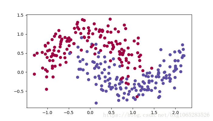
Lets use the following “moons” dataset to test the different optimization methods. (The dataset is named “moons” because the data from each of the two classes looks a bit like a crescent-shaped moon.)

We have already implemented a 3-layer neural network. You will train it with:
- Mini-batch Gradient Descent: it will call your function:
- update_parameters_with_gd()
- Mini-batch Momentum: it will call your functions:
- initialize_velocity() and update_parameters_with_momentum()
- Mini-batch Adam: it will call your functions:
- initialize_adam() and update_parameters_with_adam()
You will now run this 3 layer neural network with each of the 3 optimization methods.
5.1 - Mini-batch Gradient descent
Run the following code to see how the model does with mini-batch gradient descent.
def model(X, Y, layers_dims, optimizer, learning_rate = 0.0007, mini_batch_size = 64, beta = 0.9,
beta1 = 0.9, beta2 = 0.999, epsilon = 1e-8, num_epochs = 10000, print_cost = True):
"""
3-layer neural network model which can be run in different optimizer modes.
Arguments:
X -- input data, of shape (2, number of examples)
Y -- true "label" vector (1 for blue dot / 0 for red dot), of shape (1, number of examples)
layers_dims -- python list, containing the size of each layer
learning_rate -- the learning rate, scalar.
mini_batch_size -- the size of a mini batch
beta -- Momentum hyperparameter
beta1 -- Exponential decay hyperparameter for the past gradients estimates
beta2 -- Exponential decay hyperparameter for the past squared gradients estimates
epsilon -- hyperparameter preventing division by zero in Adam updates
num_epochs -- number of epochs
print_cost -- True to print the cost every 1000 epochs
Returns:
parameters -- python dictionary containing your updated parameters
"""
L = len(layers_dims) # number of layers in the neural networks
costs = [] # to keep track of the cost
t = 0 # initializing the counter required for Adam update
seed = 10 # For grading purposes, so that your "random" minibatches are the same as ours
# Initialize parameters
parameters = initialize_parameters(layers_dims)
# Initialize the optimizer
if optimizer == "gd":
pass # no initialization required for gradient descent
elif optimizer == "momentum":
v = initialize_velocity(parameters)
elif optimizer == "adam":
v, s = initialize_adam(parameters)
# Optimization loop
for i in range(num_epochs):
# Define the random minibatches. We increment the seed to reshuffle differently the dataset after each epoch
seed = seed + 1
minibatches = random_mini_batches(X, Y, mini_batch_size, seed)
for minibatch in minibatches:
# Select a minibatch
(minibatch_X, minibatch_Y) = minibatch
# Forward propagation
a3, caches = forward_propagation(minibatch_X, parameters)
# Compute cost
cost = compute_cost(a3, minibatch_Y)
# Backward propagation
grads = backward_propagation(minibatch_X, minibatch_Y, caches)
# Update parameters
if optimizer == "gd":
parameters = update_parameters_with_gd(parameters, grads, learning_rate)
elif optimizer == "momentum":
parameters, v = update_parameters_with_momentum(parameters, grads, v, beta, learning_rate)
elif optimizer == "adam":
t = t + 1 # Adam counter
parameters, v, s = update_parameters_with_adam(parameters, grads, v, s,
t, learning_rate, beta1, beta2, epsilon)
# Print the cost every 1000 epoch
if print_cost and i % 1000 == 0:
print ("Cost after epoch %i: %f" %(i, cost))
if print_cost and i % 100 == 0:
costs.append(cost)
# plot the cost
plt.plot(costs)
plt.ylabel('cost')
plt.xlabel('epochs (per 100)')
plt.title("Learning rate = " + str(learning_rate))
plt.show()
return parameters
train_X, train_Y = load_dataset()
# train 3-layer model
layers_dims = [train_X.shape[0], 5, 2, 1]
parameters = model(train_X, train_Y, layers_dims, optimizer = "gd")
# Predict
predictions = predict(train_X, train_Y, parameters)
# Plot decision boundary
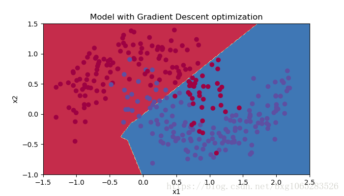
plt.title("Model with Gradient Descent optimization")
axes = plt.gca()
axes.set_xlim([-1.5,2.5])
axes.set_ylim([-1,1.5])
plot_decision_boundary(lambda x: predict_dec(parameters, x.T), train_X, train_Y)
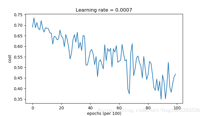
Cost after epoch 0: 0.690736
Cost after epoch 1000: 0.685273
Cost after epoch 2000: 0.647072
Cost after epoch 3000: 0.619525
Cost after epoch 4000: 0.576584
Cost after epoch 5000: 0.607243
Cost after epoch 6000: 0.529403
Cost after epoch 7000: 0.460768
Cost after epoch 8000: 0.465586
Cost after epoch 9000: 0.464518
Accuracy: 0.7966666666666666
5.2 - Mini-batch gradient descent with momentum
Run the following code to see how the model does with momentum. Because this example is relatively simple, the gains from using momemtum are small; but for more complex problems you might see bigger gains.
# train 3-layer model
layers_dims = [train_X.shape[0], 5, 2, 1]
parameters = model(train_X, train_Y, layers_dims, beta = 0.9, optimizer = "momentum")

# Predict
predictions = predict(train_X, train_Y, parameters)

# Plot decision boundary
plt.title("Model with Momentum optimization")
axes = plt.gca()
axes.set_xlim([-1.5,2.5])
axes.set_ylim([-1,1.5])
plot_decision_boundary(lambda x: predict_dec(parameters, x.T), train_X, train_Y)

Cost after epoch 0: 0.690741
Cost after epoch 1000: 0.685341
Cost after epoch 2000: 0.647145
Cost after epoch 3000: 0.619594
Cost after epoch 4000: 0.576665
Cost after epoch 5000: 0.607324
Cost after epoch 6000: 0.529476
Cost after epoch 7000: 0.460936
Cost after epoch 8000: 0.465780
Cost after epoch 9000: 0.464740
Accuracy: 0.7966666666666666

5.3 - Mini-batch with Adam mode
Run the following code to see how the model does with Adam.
# train 3-layer model
layers_dims = [train_X.shape[0], 5, 2, 1]
parameters = model(train_X, train_Y, layers_dims, optimizer = "adam")

# Predict
predictions = predict(train_X, train_Y, parameters)

# Plot decision boundary
plt.title("Model with Adam optimization")
axes = plt.gca()
axes.set_xlim([-1.5,2.5])
axes.set_ylim([-1,1.5])
plot_decision_boundary(lambda x: predict_dec(parameters, x.T), train_X, train_Y)

Cost after epoch 0: 0.690552
Cost after epoch 1000: 0.185501
Cost after epoch 2000: 0.150830
Cost after epoch 3000: 0.074454
Cost after epoch 4000: 0.125959
Cost after epoch 5000: 0.104344
Cost after epoch 6000: 0.100676
Cost after epoch 7000: 0.031652
Cost after epoch 8000: 0.111973
Cost after epoch 9000: 0.197940
Accuracy: 0.94

5.4 - Summary
Momentum usually helps, but given the small learning rate and the simplistic dataset, its impact is almost negligeable. Also, the huge oscillations you see in the cost come from the fact that some minibatches are more difficult thans others for the optimization algorithm.(动量通常是有帮助的,但由于学习速度慢,数据集简单,其影响几乎可以忽略不计。另外,在成本中看到的巨大振荡来自于这样一个事实,即一些小型机器在优化算法上比其他小机型更困难)
Adam on the other hand, clearly outperforms mini-batch gradient descent and Momentum. If you run the model for more epochs on this simple dataset, all three methods will lead to very good results. However, you’ve seen that Adam converges a lot faster.(Adam另一方面,显然胜过小批量梯度下降和动量。如果你在这个简单的数据集上运行更多时期的模型,这三种方法都会带来非常好的结果。不过,你已经看到Adam更快地收敛了)
Some advantages of Adam include:
- Relatively low memory requirements (though higher than gradient descent and gradient descent with momentum) (*
相对较低的内存需求(虽然高于梯度下降和动量梯度下降)*)
- Usually works well even with little tuning of hyperparameters (except α)(即使对超参数进行了微调,通常也能正常工作(α除外))
References:
- Adam paper: https://arxiv.org/pdf/1412.6980.pdf
附录:
demo.py
import numpy as np
import matplotlib.pyplot as plt
import scipy.io
import math
import sklearn
import sklearn.datasets

from opt_utils import load_params_and_grads, initialize_parameters, forward_propagation, backward_propagation
from opt_utils import compute_cost, predict, predict_dec, plot_decision_boundary, load_dataset
from opt_utils import update_parameters_with_gd_test_case,random_mini_batches_test_case,initialize_velocity_test_case,update_parameters_with_momentum_test_case,initialize_adam_test_case,update_parameters_with_adam_test_case
from testCases import *


# plt.rcParams['figure.figsize'] = (7.0, 4.0) # set default size of plots
# plt.rcParams['image.interpolation'] = 'nearest'
# plt.rcParams['image.cmap'] = 'gray'


def update_parameters_with_gd(parameters, grads, learning_rate):
    """
    Update parameters using one step of gradient descent

    Arguments:
    parameters -- python dictionary containing your parameters to be updated:
                    parameters['W' + str(l)] = Wl
                    parameters['b' + str(l)] = bl
    grads -- python dictionary containing your gradients to update each parameters:
                    grads['dW' + str(l)] = dWl
                    grads['db' + str(l)] = dbl
    learning_rate -- the learning rate, scalar.

    Returns:
    parameters -- python dictionary containing your updated parameters
    """

    L = len(parameters) // 2 # number of layers in the neural networks

    # Update rule for each parameter
    for l in range(L):
        ### START CODE HERE ### (approx. 2 lines)
        parameters["W" + str(l+1)] = parameters["W"+str(l+1)]-learning_rate*grads["dW"+str(l+1)]
        parameters["b" + str(l+1)] = parameters["b"+str(l+1)]-learning_rate*grads["db"+str(l+1)]
        ### END CODE HERE ###

    return parameters

def random_mini_batches(X, Y, mini_batch_size = 64, seed = 0):
    """
    Creates a list of random minibatches from (X, Y)

    Arguments:
    X -- input data, of shape (input size, number of examples)
    Y -- true "label" vector (1 for blue dot / 0 for red dot), of shape (1, number of examples)
    mini_batch_size -- size of the mini-batches, integer

    Returns:
    mini_batches -- list of synchronous (mini_batch_X, mini_batch_Y)
    """

    np.random.seed(seed)            # To make your "random" minibatches the same as ours
    m = X.shape[1]                  # number of training examples
    mini_batches = []

    # Step 1: Shuffle (X, Y)
    permutation = list(np.random.permutation(m))
    shuffled_X = X[:, permutation]
    shuffled_Y = Y[:, permutation].reshape((1,m))

    # Step 2: Partition (shuffled_X, shuffled_Y). Minus the end case.
    num_complete_minibatches = math.floor(m/mini_batch_size) # number of mini batches of size mini_batch_size in your partitionning
    for k in range(0, num_complete_minibatches):
        ### START CODE HERE ### (approx. 2 lines)
        mini_batch_X = shuffled_X[:,k * mini_batch_size : (k+1) * mini_batch_size]
        mini_batch_Y = shuffled_Y[:,k * mini_batch_size : (k+1) * mini_batch_size]
        ### END CODE HERE ###
        mini_batch = (mini_batch_X, mini_batch_Y)
        mini_batches.append(mini_batch)

    # Handling the end case (last mini-batch < mini_batch_size)
    if m % mini_batch_size != 0:
        ### START CODE HERE ### (approx. 2 lines)
        mini_batch_X = shuffled_X[:,num_complete_minibatches * mini_batch_size:]
        mini_batch_Y = shuffled_Y[:,num_complete_minibatches * mini_batch_size:]
        ### END CODE HERE ###
        mini_batch = (mini_batch_X, mini_batch_Y)
        mini_batches.append(mini_batch)

    return mini_batches

def initialize_velocity(parameters):
    """
    Initializes the velocity as a python dictionary with:
                - keys: "dW1", "db1", ..., "dWL", "dbL"
                - values: numpy arrays of zeros of the same shape as the corresponding gradients/parameters.
    Arguments:
    parameters -- python dictionary containing your parameters.
                    parameters['W' + str(l)] = Wl
                    parameters['b' + str(l)] = bl

    Returns:
    v -- python dictionary containing the current velocity.
                    v['dW' + str(l)] = velocity of dWl
                    v['db' + str(l)] = velocity of dbl
    """

    L = len(parameters) // 2 # number of layers in the neural networks
    v = {}

    # Initialize velocity
    for l in range(L):
        ### START CODE HERE ### (approx. 2 lines)
        v["dW" + str(l+1)] = np.zeros(parameters["W" + str(l+1)].shape)
        v["db" + str(l+1)] = np.zeros(parameters["b" + str(l+1)].shape)
        ### END CODE HERE ###

    return v

def update_parameters_with_momentum(parameters, grads, v, beta, learning_rate):
    """
    Update parameters using Momentum

    Arguments:
    parameters -- python dictionary containing your parameters:
                    parameters['W' + str(l)] = Wl
                    parameters['b' + str(l)] = bl
    grads -- python dictionary containing your gradients for each parameters:
                    grads['dW' + str(l)] = dWl
                    grads['db' + str(l)] = dbl
    v -- python dictionary containing the current velocity:
                    v['dW' + str(l)] = ...
                    v['db' + str(l)] = ...
    beta -- the momentum hyperparameter, scalar
    learning_rate -- the learning rate, scalar

    Returns:
    parameters -- python dictionary containing your updated parameters
    v -- python dictionary containing your updated velocities
    """

    L = len(parameters) // 2 # number of layers in the neural networks

    # Momentum update for each parameter
    for l in range(L):

        ### START CODE HERE ### (approx. 4 lines)
        # compute velocities
        v["dW" + str(l+1)] = np.dot(beta,v["dW"+str(l+1)]) + np.dot(1-beta,grads["dW"+str(l+1)])
        v["db" + str(l+1)] = np.dot(beta,v["db"+str(l+1)]) + np.dot(1-beta,grads["db"+str(l+1)])
        # update parameters
        parameters["W" + str(l+1)] = parameters["W" + str(l+1)] - learning_rate*v["dW" + str(l+1)]
        parameters["b" + str(l+1)] = parameters["b" + str(l+1)] - learning_rate*v["db" + str(l+1)]
        ### END CODE HERE ###

    return parameters, v

def initialize_adam(parameters) :
    """
    Initializes v and s as two python dictionaries with:
                - keys: "dW1", "db1", ..., "dWL", "dbL"
                - values: numpy arrays of zeros of the same shape as the corresponding gradients/parameters.

    Arguments:
    parameters -- python dictionary containing your parameters.
                    parameters["W" + str(l)] = Wl
                    parameters["b" + str(l)] = bl

    Returns:
    v -- python dictionary that will contain the exponentially weighted average of the gradient.
                    v["dW" + str(l)] = ...
                    v["db" + str(l)] = ...
    s -- python dictionary that will contain the exponentially weighted average of the squared gradient.
                    s["dW" + str(l)] = ...
                    s["db" + str(l)] = ...

    """

    L = len(parameters) // 2 # number of layers in the neural networks
    v = {}
    s = {}

    # Initialize v, s. Input: "parameters". Outputs: "v, s".
    for l in range(L):
    ### START CODE HERE ### (approx. 4 lines)
        v["dW" + str(l+1)] = np.zeros(parameters["W" + str(l+1)].shape)
        v["db" + str(l+1)] = np.zeros(parameters["b" + str(l+1)].shape)
        s["dW" + str(l+1)] = np.zeros(parameters["W" + str(l+1)].shape)
        s["db" + str(l+1)] = np.zeros(parameters["b" + str(l+1)].shape)
    ### END CODE HERE ###

    return v, s

def update_parameters_with_adam(parameters, grads, v, s, t, learning_rate = 0.01,
                                beta1 = 0.9, beta2 = 0.999,  epsilon = 1e-8):
    """
    Update parameters using Adam

    Arguments:
    parameters -- python dictionary containing your parameters:
                    parameters['W' + str(l)] = Wl
                    parameters['b' + str(l)] = bl
    grads -- python dictionary containing your gradients for each parameters:
                    grads['dW' + str(l)] = dWl
                    grads['db' + str(l)] = dbl
    v -- Adam variable, moving average of the first gradient, python dictionary
    s -- Adam variable, moving average of the squared gradient, python dictionary
    learning_rate -- the learning rate, scalar.
    beta1 -- Exponential decay hyperparameter for the first moment estimates
    beta2 -- Exponential decay hyperparameter for the second moment estimates
    epsilon -- hyperparameter preventing division by zero in Adam updates

    Returns:
    parameters -- python dictionary containing your updated parameters
    v -- Adam variable, moving average of the first gradient, python dictionary
    s -- Adam variable, moving average of the squared gradient, python dictionary
    """

    L = len(parameters) // 2                 # number of layers in the neural networks
    v_corrected = {}                         # Initializing first moment estimate, python dictionary
    s_corrected = {}                         # Initializing second moment estimate, python dictionary

    # Perform Adam update on all parameters
    for l in range(L):
        # Moving average of the gradients. Inputs: "v, grads, beta1". Output: "v".
        ### START CODE HERE ### (approx. 2 lines)
        v["dW" + str(l+1)] = beta1 * v["dW" + str(l+1)] + (1 - beta1) * grads["dW" + str(l+1)]
        v["db" + str(l+1)] = beta1 * v["db" + str(l+1)] + (1 - beta1) * grads["db" + str(l+1)]
        ### END CODE HERE ###

        # Compute bias-corrected first moment estimate. Inputs: "v, beta1, t". Output: "v_corrected".
        ### START CODE HERE ### (approx. 2 lines)
        v_corrected["dW" + str(l + 1)] = v["dW" + str(l + 1)]/(1-(beta1)**t)
        v_corrected["db" + str(l + 1)] = v["db" + str(l + 1)]/(1-(beta1)**t)
        ### END CODE HERE ###

        # Moving average of the squared gradients. Inputs: "s, grads, beta2". Output: "s".
        ### START CODE HERE ### (approx. 2 lines)
        s["dW" + str(l+1)] = beta2 * s["dW" + str(l+1)] + (1 - beta2) * grads["dW" + str(l+1)]**2
        s["db" + str(l+1)] = beta2 * s["db" + str(l+1)] + (1 - beta2) * grads["db" + str(l+1)]**2
        ### END CODE HERE ###

        # Compute bias-corrected second raw moment estimate. Inputs: "s, beta2, t". Output: "s_corrected".
        ### START CODE HERE ### (approx. 2 lines)
        s_corrected["dW" + str(l + 1)] =s["dW" + str(l + 1)]/(1-(beta2)**t)
        s_corrected["db" + str(l + 1)] = s["db" + str(l + 1)]/(1-(beta2)**t)
        ### END CODE HERE ###

        # Update parameters. Inputs: "parameters, learning_rate, v_corrected, s_corrected, epsilon". Output: "parameters".
        ### START CODE HERE ### (approx. 2 lines)
        parameters["W" + str(l + 1)] = parameters["W" + str(l + 1)]-learning_rate*(v_corrected["dW" + str(l + 1)]/np.sqrt( s_corrected["dW" + str(l + 1)]+epsilon))
        parameters["b" + str(l + 1)] = parameters["b" + str(l + 1)]-learning_rate*(v_corrected["db" + str(l + 1)]/np.sqrt( s_corrected["db" + str(l + 1)]+epsilon))
        ### END CODE HERE ###

    return parameters, v, s

def model(X, Y, layers_dims, optimizer, learning_rate = 0.0007, mini_batch_size = 64, beta = 0.9,
          beta1 = 0.9, beta2 = 0.999,  epsilon = 1e-8, num_epochs = 10000, print_cost = True):
    """
    3-layer neural network model which can be run in different optimizer modes.

    Arguments:
    X -- input data, of shape (2, number of examples)
    Y -- true "label" vector (1 for blue dot / 0 for red dot), of shape (1, number of examples)
    layers_dims -- python list, containing the size of each layer
    learning_rate -- the learning rate, scalar.
    mini_batch_size -- the size of a mini batch
    beta -- Momentum hyperparameter
    beta1 -- Exponential decay hyperparameter for the past gradients estimates
    beta2 -- Exponential decay hyperparameter for the past squared gradients estimates
    epsilon -- hyperparameter preventing division by zero in Adam updates
    num_epochs -- number of epochs
    print_cost -- True to print the cost every 1000 epochs

    Returns:
    parameters -- python dictionary containing your updated parameters
    """

    L = len(layers_dims)             # number of layers in the neural networks
    costs = []                       # to keep track of the cost
    t = 0                            # initializing the counter required for Adam update
    seed = 10                        # For grading purposes, so that your "random" minibatches are the same as ours

    # Initialize parameters
    parameters = initialize_parameters(layers_dims)

    # Initialize the optimizer
    if optimizer == "gd":
        pass # no initialization required for gradient descent
    elif optimizer == "momentum":
        v = initialize_velocity(parameters)
    elif optimizer == "adam":
        v, s = initialize_adam(parameters)

    # Optimization loop
    for i in range(num_epochs):

        # Define the random minibatches. We increment the seed to reshuffle differently the dataset after each epoch
        seed = seed + 1
        minibatches = random_mini_batches(X, Y, mini_batch_size, seed)

        for minibatch in minibatches:

            # Select a minibatch
            (minibatch_X, minibatch_Y) = minibatch

            # Forward propagation
            a3, caches = forward_propagation(minibatch_X, parameters)

            # Compute cost
            cost = compute_cost(a3, minibatch_Y)

            # Backward propagation
            grads = backward_propagation(minibatch_X, minibatch_Y, caches)

            # Update parameters
            if optimizer == "gd":
                parameters = update_parameters_with_gd(parameters, grads, learning_rate)
            elif optimizer == "momentum":
                parameters, v = update_parameters_with_momentum(parameters, grads, v, beta, learning_rate)
            elif optimizer == "adam":
                t = t + 1 # Adam counter
                parameters, v, s = update_parameters_with_adam(parameters, grads, v, s,
                                                               t, learning_rate, beta1, beta2,  epsilon)

        # Print the cost every 1000 epoch
        if print_cost and i % 1000 == 0:
            print ("Cost after epoch %i: %f" %(i, cost))
        if print_cost and i % 100 == 0:
            costs.append(cost)

    # plot the cost
    plt.plot(costs)
    plt.ylabel('cost')
    plt.xlabel('epochs (per 100)')
    plt.title("Learning rate = " + str(learning_rate))
    plt.show()

    return parameters

train_X, train_Y = load_dataset()
# train 3-layer model
layers_dims = [train_X.shape[0], 5, 2, 1]
parameters = model(train_X, train_Y, layers_dims, optimizer = "adam")

# Predict
predictions = predict(train_X, train_Y, parameters)

# Plot decision boundary
plt.title("Model with Gradient Descent optimization")
axes = plt.gca()
axes.set_xlim([-1.5,2.5])
axes.set_ylim([-1,1.5])
plot_decision_boundary(lambda x: predict_dec(parameters, x.T), train_X, train_Y)
opt_utils.py
import numpy as np
import matplotlib.pyplot as plt
import h5py
import scipy.io
import sklearn
import sklearn.datasets

def sigmoid(x):
    """
    Compute the sigmoid of x

    Arguments:
    x -- A scalar or numpy array of any size.

    Return:
    s -- sigmoid(x)
    """
    s = 1/(1+np.exp(-x))
    return s

def relu(x):
    """
    Compute the relu of x

    Arguments:
    x -- A scalar or numpy array of any size.

    Return:
    s -- relu(x)
    """
    s = np.maximum(0,x)

    return s

def load_params_and_grads(seed=1):
    np.random.seed(seed)
    W1 = np.random.randn(2,3)
    b1 = np.random.randn(2,1)
    W2 = np.random.randn(3,3)
    b2 = np.random.randn(3,1)

    dW1 = np.random.randn(2,3)
    db1 = np.random.randn(2,1)
    dW2 = np.random.randn(3,3)
    db2 = np.random.randn(3,1)

    return W1, b1, W2, b2, dW1, db1, dW2, db2


def initialize_parameters(layer_dims):
    """
    Arguments:
    layer_dims -- python array (list) containing the dimensions of each layer in our network

    Returns:
    parameters -- python dictionary containing your parameters "W1", "b1", ..., "WL", "bL":
                    W1 -- weight matrix of shape (layer_dims[l], layer_dims[l-1])
                    b1 -- bias vector of shape (layer_dims[l], 1)
                    Wl -- weight matrix of shape (layer_dims[l-1], layer_dims[l])
                    bl -- bias vector of shape (1, layer_dims[l])

    Tips:
    - For example: the layer_dims for the "Planar Data classification model" would have been [2,2,1].
    This means W1's shape was (2,2), b1 was (1,2), W2 was (2,1) and b2 was (1,1). Now you have to generalize it!
    - In the for loop, use parameters['W' + str(l)] to access Wl, where l is the iterative integer.
    """

    np.random.seed(3)
    parameters = {}
    L = len(layer_dims) # number of layers in the network

    for l in range(1, L):
        parameters['W' + str(l)] = np.random.randn(layer_dims[l], layer_dims[l-1])*  np.sqrt(2.0 / layer_dims[l-1])  #请注意这里的2.0很重要
        parameters['b' + str(l)] = np.zeros((layer_dims[l], 1))

        assert(parameters['W' + str(l)].shape == layer_dims[l], layer_dims[l-1])
        assert(parameters['W' + str(l)].shape == layer_dims[l], 1)

    return parameters


def compute_cost(a3, Y):

    """
    Implement the cost function

    Arguments:
    a3 -- post-activation, output of forward propagation
    Y -- "true" labels vector, same shape as a3

    Returns:
    cost - value of the cost function
    """
    m = Y.shape[1]

    logprobs = np.multiply(-np.log(a3),Y) + np.multiply(-np.log(1 - a3), 1 - Y)
    cost = 1./m * np.sum(logprobs)

    return cost

def forward_propagation(X, parameters):
    """
    Implements the forward propagation (and computes the loss) presented in Figure 2.

    Arguments:
    X -- input dataset, of shape (input size, number of examples)
    parameters -- python dictionary containing your parameters "W1", "b1", "W2", "b2", "W3", "b3":
                    W1 -- weight matrix of shape ()
                    b1 -- bias vector of shape ()
                    W2 -- weight matrix of shape ()
                    b2 -- bias vector of shape ()
                    W3 -- weight matrix of shape ()
                    b3 -- bias vector of shape ()

    Returns:
    loss -- the loss function (vanilla logistic loss)
    """

    # retrieve parameters
    W1 = parameters["W1"]
    b1 = parameters["b1"]
    W2 = parameters["W2"]
    b2 = parameters["b2"]
    W3 = parameters["W3"]
    b3 = parameters["b3"]

    # LINEAR -> RELU -> LINEAR -> RELU -> LINEAR -> SIGMOID
    z1 = np.dot(W1, X) + b1
    a1 = relu(z1)
    z2 = np.dot(W2, a1) + b2
    a2 = relu(z2)
    z3 = np.dot(W3, a2) + b3
    a3 = sigmoid(z3)

    cache = (z1, a1, W1, b1, z2, a2, W2, b2, z3, a3, W3, b3)

    return a3, cache

def backward_propagation(X, Y, cache):
    """
    Implement the backward propagation presented in figure 2.

    Arguments:
    X -- input dataset, of shape (input size, number of examples)
    Y -- true "label" vector (containing 0 if cat, 1 if non-cat)
    cache -- cache output from forward_propagation()

    Returns:
    gradients -- A dictionary with the gradients with respect to each parameter, activation and pre-activation variables
    """
    m = X.shape[1]
    (z1, a1, W1, b1, z2, a2, W2, b2, z3, a3, W3, b3) = cache

    dz3 = 1./m * (a3 - Y)
    dW3 = np.dot(dz3, a2.T)
    db3 = np.sum(dz3, axis=1, keepdims = True)

    da2 = np.dot(W3.T, dz3)
    dz2 = np.multiply(da2, np.int64(a2 > 0))
    dW2 = np.dot(dz2, a1.T)
    db2 = np.sum(dz2, axis=1, keepdims = True)

    da1 = np.dot(W2.T, dz2)
    dz1 = np.multiply(da1, np.int64(a1 > 0))
    dW1 = np.dot(dz1, X.T)
    db1 = np.sum(dz1, axis=1, keepdims = True)

    gradients = {"dz3": dz3, "dW3": dW3, "db3": db3,
                 "da2": da2, "dz2": dz2, "dW2": dW2, "db2": db2,
                 "da1": da1, "dz1": dz1, "dW1": dW1, "db1": db1}

    return gradients

def predict(X, y, parameters):
    """
    This function is used to predict the results of a  n-layer neural network.

    Arguments:
    X -- data set of examples you would like to label
    parameters -- parameters of the trained model

    Returns:
    p -- predictions for the given dataset X
    """

    m = X.shape[1]
    p = np.zeros((1,m), dtype = np.int)

    # Forward propagation
    a3, caches = forward_propagation(X, parameters)

    # convert probas to 0/1 predictions
    for i in range(0, a3.shape[1]):
        if a3[0,i] > 0.5:
            p[0,i] = 1
        else:
            p[0,i] = 0

    # print results

    #print ("predictions: " + str(p[0,:]))
    #print ("true labels: " + str(y[0,:]))
    print("Accuracy: "  + str(np.mean((p[0,:] == y[0,:]))))

    return p

def load_2D_dataset():
    data = scipy.io.loadmat('data.mat')
    train_X = data['X'].T
    train_Y = data['y'].T
    test_X = data['Xval'].T
    test_Y = data['yval'].T

    plt.scatter(train_X[0, :], train_X[1, :], c=train_Y, s=40);

    return train_X, train_Y, test_X, test_Y

def plot_decision_boundary(model, X, y):
    # Set min and max values and give it some padding
    x_min, x_max = X[0, :].min() - 1, X[0, :].max() + 1
    y_min, y_max = X[1, :].min() - 1, X[1, :].max() + 1
    h = 0.01
    # Generate a grid of points with distance h between them
    xx, yy = np.meshgrid(np.arange(x_min, x_max, h), np.arange(y_min, y_max, h))
    # Predict the function value for the whole grid
    Z = model(np.c_[xx.ravel(), yy.ravel()])
    Z = Z.reshape(xx.shape)
    # Plot the contour and training examples
    plt.contourf(xx, yy, Z)
    plt.ylabel('x2')
    plt.xlabel('x1')
    plt.scatter(X[0, :], X[1, :], c=y)
    plt.show()

def predict_dec(parameters, X):
    """
    Used for plotting decision boundary.

    Arguments:
    parameters -- python dictionary containing your parameters
    X -- input data of size (m, K)

    Returns
    predictions -- vector of predictions of our model (red: 0 / blue: 1)
    """

    # Predict using forward propagation and a classification threshold of 0.5
    a3, cache = forward_propagation(X, parameters)
    predictions = (a3 > 0.5)
    return predictions

def load_dataset():
    np.random.seed(3)
    train_X, train_Y = sklearn.datasets.make_moons(n_samples=300, noise=.2) #300 #0.2
    # Visualize the data
    #plt.scatter(train_X[:, 0], train_X[:, 1], c=train_Y, s=40);
    train_X = train_X.T
    train_Y = train_Y.reshape((1, train_Y.shape[0]))

    return train_X, train_Y

def update_parameters_with_gd_test_case():
    np.random.seed(1)
    learning_rate = 0.01
    W1 = np.random.randn(2,3)
    b1 = np.random.randn(2,1)
    W2 = np.random.randn(3,3)
    b2 = np.random.randn(3,1)

    dW1 = np.random.randn(2,3)
    db1 = np.random.randn(2,1)
    dW2 = np.random.randn(3,3)
    db2 = np.random.randn(3,1)

    parameters = {"W1": W1, "b1": b1, "W2": W2, "b2": b2}
    grads = {"dW1": dW1, "db1": db1, "dW2": dW2, "db2": db2}

    return parameters, grads, learning_rate

"""
def update_parameters_with_sgd_checker(function, inputs, outputs):
    if function(inputs) == outputs:
        print("Correct")
    else:
        print("Incorrect")
"""

def random_mini_batches_test_case():
    np.random.seed(1)
    mini_batch_size = 64
    X = np.random.randn(12288, 148)
    Y = np.random.randn(1, 148) < 0.5
    return X, Y, mini_batch_size

def initialize_velocity_test_case():
    np.random.seed(1)
    W1 = np.random.randn(2,3)
    b1 = np.random.randn(2,1)
    W2 = np.random.randn(3,3)
    b2 = np.random.randn(3,1)
    parameters = {"W1": W1, "b1": b1, "W2": W2, "b2": b2}
    return parameters

def update_parameters_with_momentum_test_case():
    np.random.seed(1)
    W1 = np.random.randn(2,3)
    b1 = np.random.randn(2,1)
    W2 = np.random.randn(3,3)
    b2 = np.random.randn(3,1)

    dW1 = np.random.randn(2,3)
    db1 = np.random.randn(2,1)
    dW2 = np.random.randn(3,3)
    db2 = np.random.randn(3,1)
    parameters = {"W1": W1, "b1": b1, "W2": W2, "b2": b2}
    grads = {"dW1": dW1, "db1": db1, "dW2": dW2, "db2": db2}
    v = {'dW1': np.array([[ 0.,  0.,  0.],
        [ 0.,  0.,  0.]]), 'dW2': np.array([[ 0.,  0.,  0.],
        [ 0.,  0.,  0.],
        [ 0.,  0.,  0.]]), 'db1': np.array([[ 0.],
        [ 0.]]), 'db2': np.array([[ 0.],
        [ 0.],
        [ 0.]])}
    return parameters, grads, v

def initialize_adam_test_case():
    np.random.seed(1)
    W1 = np.random.randn(2,3)
    b1 = np.random.randn(2,1)
    W2 = np.random.randn(3,3)
    b2 = np.random.randn(3,1)
    parameters = {"W1": W1, "b1": b1, "W2": W2, "b2": b2}
    return parameters

def update_parameters_with_adam_test_case():
    np.random.seed(1)
    v, s = ({'dW1': np.array([[ 0.,  0.,  0.],
         [ 0.,  0.,  0.]]), 'dW2': np.array([[ 0.,  0.,  0.],
         [ 0.,  0.,  0.],
         [ 0.,  0.,  0.]]), 'db1': np.array([[ 0.],
         [ 0.]]), 'db2': np.array([[ 0.],
         [ 0.],
         [ 0.]])}, {'dW1': np.array([[ 0.,  0.,  0.],
         [ 0.,  0.,  0.]]), 'dW2': np.array([[ 0.,  0.,  0.],
         [ 0.,  0.,  0.],
         [ 0.,  0.,  0.]]), 'db1': np.array([[ 0.],
         [ 0.]]), 'db2': np.array([[ 0.],
         [ 0.],
         [ 0.]])})
    W1 = np.random.randn(2,3)
    b1 = np.random.randn(2,1)
    W2 = np.random.randn(3,3)
    b2 = np.random.randn(3,1)

    dW1 = np.random.randn(2,3)
    db1 = np.random.randn(2,1)
    dW2 = np.random.randn(3,3)
    db2 = np.random.randn(3,1)

    parameters = {"W1": W1, "b1": b1, "W2": W2, "b2": b2}
    grads = {"dW1": dW1, "db1": db1, "dW2": dW2, "db2": db2}

    return parameters, grads, v, s