【SciKit-Learn学习笔记】5：核SVM分类和预测乳腺癌数据集

学习《scikit-learn机器学习》时的一些实践。

常用参数

参数`C`

SVM分类器svm.SVC()中的参数C即SVM所优化的目标函数
$argmin \left( ||\pmb{w}||^2+R \sum_{i=1}^m \varepsilon_i \right)$
中，松弛系数 $\varepsilon$ 求和项的系数 $R$ 。

松弛系数 $\varepsilon_i$ 表征了数据样本 $x^{(i)}$ 违反最大间距规则的程度。对大部分满足约束条件的样本，其松弛系数 $\varepsilon_i$ 为0；而对不满足约束条件的样本，其松弛系数 $\varepsilon_i$ 是大于0的。

所以松弛系数的求和项系数 $R$ 就是对违反最大间距规则的样本的惩罚力度，惩罚越大越不能容忍有样本不满足约束条件。这一项类似于Logistic回归中引入正则化项，都是为了减少overfitting。

参数`degree`

在多项式核中使用，表示使用的多项式的阶数。

参数`gamma`

官方文档里的原话是：

Kernel coefficient for ‘rbf’, ‘poly’ and ‘sigmoid’. If gamma is ‘auto’ then 1/n_features will be used instead.

对于多项式核，它是多项式核函数
$K\left(\pmb{x}^{(i)},\pmb{x}^{(j)}\right)=\left(\gamma \pmb{x}^{(i)T} \pmb{x}^{(j)} + c\right)^n$
中的 $\gamma$ 。

对于高斯核，它是径向基函数
$K\left(\pmb{x}^{(i)},\pmb{x}^{(j)}\right)=exp\left(-\frac{\left(\pmb{x}^{(i)}-\pmb{x}^{(j)}\right)^2}{2\sigma^2}\right)$
中的 $\frac{1}{2\sigma^2}$ 。

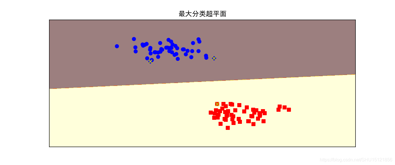
绘制最大分类超平面

打x号的点是支持向量。

from sklearn import svm
from sklearn.datasets import make_blobs
from matplotlib import pyplot as plt
import numpy as np


# 绘制分类超平面,其中X是有两个特征的,所以实际绘制出来就是在平面上的不同类别区域用不同颜色标记
# 这里h是采样步长,draw_sv指示是否绘制支持向量
def plot_hyperplane(clf, X, y,
                    h=0.02,
                    draw_sv=True,
                    title='hyperplan'):
    # 绘制的区间,x轴和y轴都从最小值-1到最大值+1
    x_min, x_max = X[:, 0].min() - 1, X[:, 0].max() + 1
    y_min, y_max = X[:, 1].min() - 1, X[:, 1].max() + 1
    # 使用np.meshgrid()扩充为两轴的所有可能取值的组合
    xx, yy = np.meshgrid(np.arange(x_min, x_max, h),
                         np.arange(y_min, y_max, h))

    plt.title(title)
    plt.xlim(xx.min(), xx.max())
    plt.ylim(yy.min(), yy.max())
    plt.xticks(())
    plt.yticks(())

    # np.ravel()将采样点的xy坐标摊平,使用np.c_将其按列组合成[[x y][x y]...]的坐标点形式
    Z = clf.predict(np.c_[xx.ravel(), yy.ravel()])
    # 用绘制等高线图的方式来绘制不同类别为不同颜色(等高线图上同一高度为同一颜色)
    Z = Z.reshape(xx.shape)
    plt.contourf(xx, yy, Z, cmap='hot', alpha=0.5)

    # 不同类(标签)展示在图上的的标记和颜色
    markers = ['o', 's', '^']
    colors = ['b', 'r', 'c']
    # 可能的类(标签)取值
    labels = np.unique(y)
    # 对于每种标签取值
    for label in labels:
        # 绘制相应的样本点,使用自己的标记和颜色
        plt.scatter(X[y == label][:, 0],
                    X[y == label][:, 1],
                    c=colors[label],
                    marker=markers[label])
    # 绘制支持向量
    if draw_sv:
        # 用该方式可以直接取出支持向量是哪些点
        sv = clf.support_vectors_
        # 绘制为白色'x',这样就会贴在之前的有色点上了
        plt.scatter(sv[:, 0], sv[:, 1], c='y', marker='x')


if __name__ == '__main__':
    # 生成聚类样本100个,特征数为2(默认n_features=2),类别数为2,标准差0.3,随机种子设为0
    X, y = make_blobs(n_samples=100, centers=2, random_state=0, cluster_std=0.3)
    # print(X,y)

    clf = svm.SVC(kernel='linear', C=1.0)
    clf.fit(X, y)

    plt.figure(figsize=(12, 4), dpi=144)
    plot_hyperplane(clf, X, y, h=0.01, title="最大分类超平面")
    plt.show()

运行结果：
在这里插入图片描述

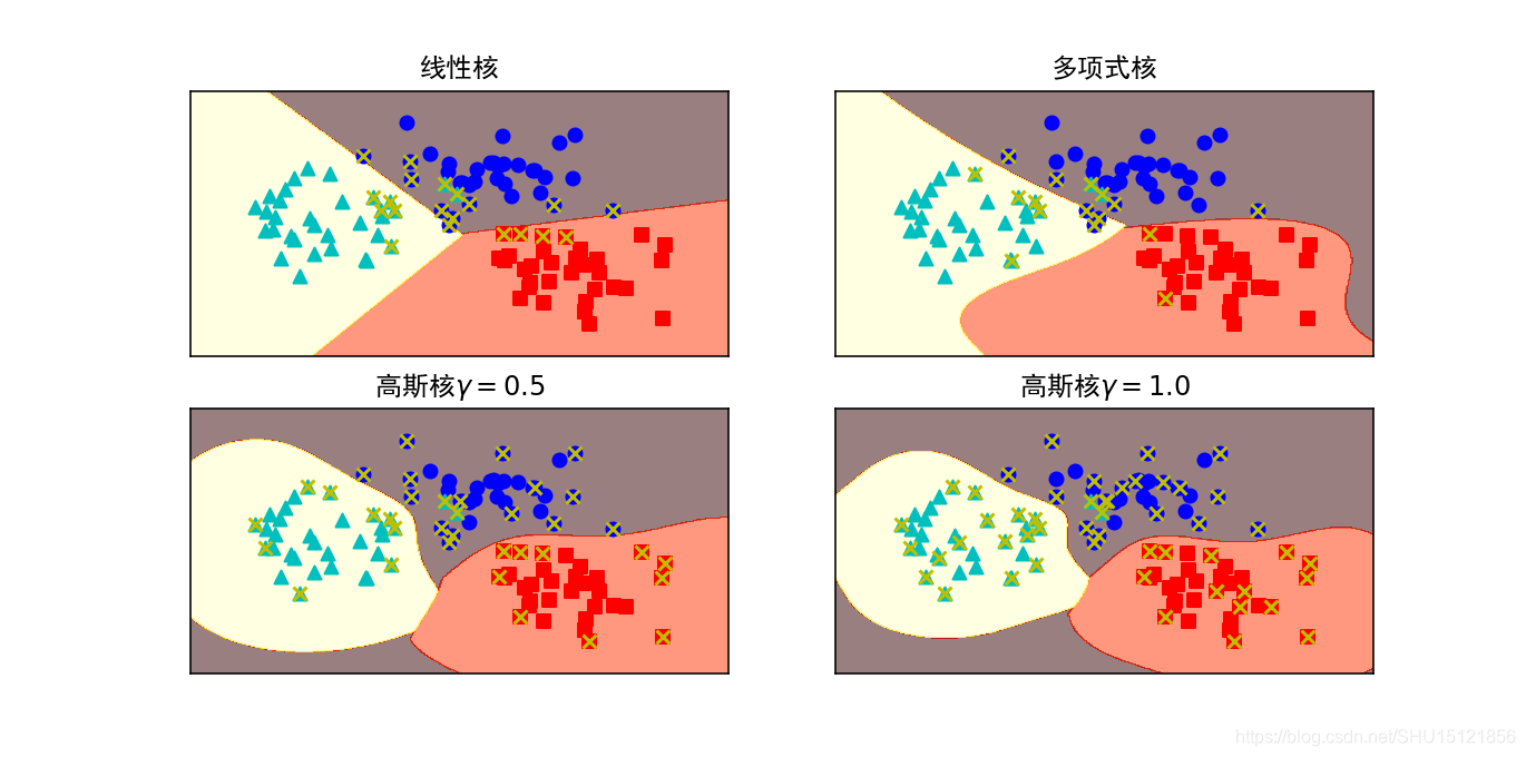
比较三种核SVM的分类面

from sklearn import svm
from sklearn.datasets import make_blobs
from matplotlib import pyplot as plt
from z8.svc2 import plot_hyperplane

X, y = make_blobs(n_samples=100, centers=3, random_state=0, cluster_std=0.8)
# 线性核
clf_linear = svm.SVC(C=1.0, kernel='linear')
# 多项式核
clf_poly = svm.SVC(C=1.0, kernel='poly', degree=3)
# 高斯核(RBF核)
clf_rbf = svm.SVC(C=1.0, kernel='rbf', gamma=0.5)
clf_rbf2 = svm.SVC(C=1.0, kernel='rbf', gamma=1.0)

plt.figure(figsize=(10, 10), dpi=144)

clfs = [clf_linear, clf_poly, clf_rbf, clf_rbf2]
titles = ["线性核", "多项式核", "高斯核$\gamma=0.5$", "高斯核$\gamma=1.0$"]

# 分别训练模型并绘制分类面.注意这里用zip组成一个个元组组成的对象
for clf, i in zip(clfs, range(len(titles))):
    clf.fit(X, y)
    plt.subplot(2, 2, i + 1)
    plot_hyperplane(clf, X, y, title=titles[i])
plt.show()

运行结果：
在这里插入图片描述

预测乳腺癌数据集

这里在最后一部分（循环中调用plot_learning_curve()）总是会有反复调用这个文件自己的奇怪现象，全部放到函数里就好了，还不清楚为什么会有这种情况。

from sklearn.datasets import load_breast_cancer
from sklearn.model_selection import train_test_split
from sklearn.svm import SVC
from z7.titanic import plot_curve  # 绘制score随参数变化的曲线
import numpy as np
from sklearn.model_selection import GridSearchCV
from matplotlib import pyplot as plt
from z3.learning_curve import plot_learning_curve  # 绘制学习曲线
from sklearn.model_selection import ShuffleSplit

'''
SVM对乳腺癌数据集做分类
这里全部需要放在函数里调用,不然会来回调用这个文件自己(还不清楚为什么,这次不是文件重名的问题)
'''


def init():
    global X, y, X_train, y_train, X_test, y_test
    cancer = load_breast_cancer()
    X = cancer.data
    y = cancer.target
    print("shape:{},阳性样本数:{},阴性样本数{}".format(X.shape, y[y == 1].shape[0], y[y == 0].shape[0]))
    X_train, X_test, y_train, y_test = train_test_split(X, y, test_size=0.2)


if __name__ == '__main__':
    init()
    # 高斯核的SVM模型很复杂,在如此小的数据集上造成了过拟合
    clf = SVC(C=1.0, kernel='rbf', gamma=1.0)
    clf.fit(X_train, y_train)
    train_score = clf.score(X_train, y_train)
    test_score = clf.score(X_test, y_test)
    print("train score:{},test score:{}".format(train_score, test_score))

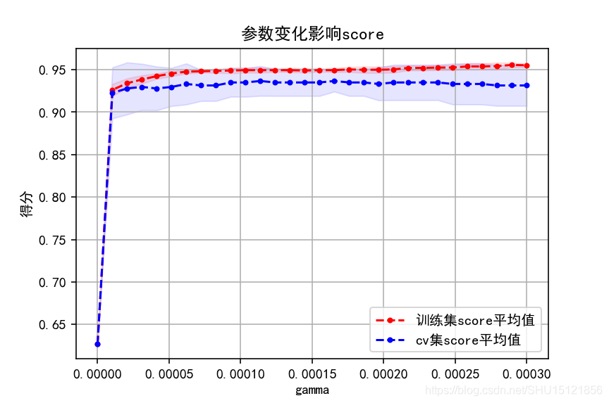
    # 获取gamma参数在一个范围集合中的最优值
    gammas = np.linspace(0, 0.0003, 30)
    param_grid = {'gamma': gammas}
    clf = GridSearchCV(SVC(), param_grid, cv=5, return_train_score=True)
    clf.fit(X, y)
    print("最优参数:{},对应score:{}".format(clf.best_params_, clf.best_score_))
    # 绘制score随着参数变化的曲线
    plot_curve(gammas, clf.cv_results_, xlabel='gamma')
    plt.show()

    # 绘制学习曲线以观察模型拟合情况
    cv = ShuffleSplit(n_splits=10, test_size=0.2, random_state=0)
    title = "高斯核SVM的学习曲线"
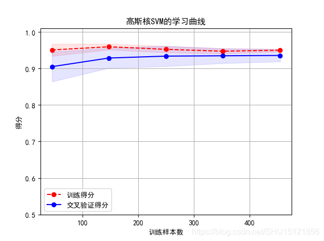
    plot_learning_curve(SVC(C=1.0, kernel='rbf', gamma=0.0001), title, X, y, ylim=(0.5, 1.01), cv=cv)
    plt.show()

    # 使用二阶多项式核
    clf = SVC(C=1.0, kernel='poly', degree=2)
    clf.fit(X_train, y_train)
    train_score = clf.score(X_train, y_train)
    test_score = clf.score(X_test, y_test)
    print("train score:{},test score:{}".format(train_score, test_score))

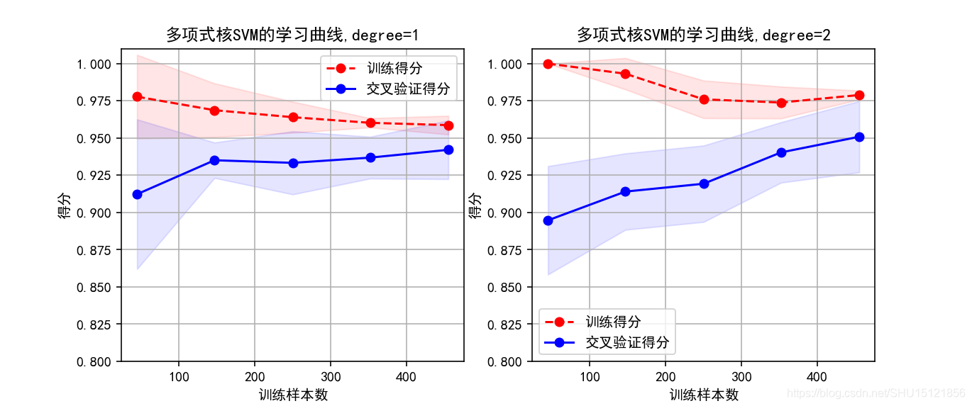
    # 对比一阶多项式和二阶多项式的学习曲线
    cv = ShuffleSplit(n_splits=5, test_size=0.2, random_state=0)
    title = "多项式核SVM的学习曲线,degree={}"
    degrees = [1, 2]
    plt.figure(figsize=(12, 4), dpi=144)
    for i in range(len(degrees)):
        plt.subplot(1, len(degrees), i + 1)
        # 这里n_jobs将传入learning_curve(),为并行运行的作业数
        plt = plot_learning_curve(SVC(C=1.0, kernel='poly', degree=degrees[i]), title.format(degrees[i]), X, y,
                                  ylim=(0.8, 1.01), cv=cv, n_jobs=4)
    plt.show()

运行结果：

shape:(569, 30),阳性样本数:357,阴性样本数212
train score:1.0,test score:0.6052631578947368
最优参数:{'gamma': 0.00011379310344827585},对应score:0.9367311072056239

从下面的图中可以看到，从gamma=0.0001之后逐渐发生了过拟合，因为训练集score在提升，而cv集score在下降。
在这里插入图片描述
从下面这张学习曲线图上可以看到用上面找到的参数 gamma=0.0001效果就比较好，试改成gamma=0.1可以看到明显的过拟合。

train score:0.9692307692307692,test score:0.9385964912280702

二阶多项式核SVM的拟合效果更好，相比一阶多项式核，其训练集和cv集上的score都有提升，不过训练代价很高。
在这里插入图片描述