#属性域
1.示例代码号码
2.块厚度1 - 10
3.细胞大小的一致性1 - 10
4.电池形状的均匀性1 - 10
5.边缘附着力1 - 10
6.单个上皮细胞大小1 - 10
7.裸核1 - 10
8.平淡的染色质1 - 10
9.正常核仁1 - 10
10.有丝分裂1 - 10
11.分类:(2为良性,4为恶性)
这是一个乳腺癌的数据集,主要通过训练来分出是否患有乳腺癌
1.1 导入类库
In [2]:
# 导入类库
from pandas import read_csv
import pandas as pd
from sklearn import datasets
from pandas.plotting import scatter_matrix
from matplotlib import pyplot
from sklearn.model_selection import train_test_split
from sklearn.model_selection import KFold
from sklearn.model_selection import cross_val_score
from sklearn.metrics import classification_report
from sklearn.metrics import confusion_matrix
from sklearn.metrics import accuracy_score
from sklearn.linear_model import LogisticRegression
from sklearn.tree import DecisionTreeClassifier
from sklearn.discriminant_analysis import LinearDiscriminantAnalysis
from sklearn.neighbors import KNeighborsClassifier
from sklearn.naive_bayes import GaussianNB
from sklearn.svm import SVC
from sklearn.preprocessing import LabelEncoder
from sklearn.linear_model import LogisticRegression

import numpy as np
import matplotlib.pyplot as plt
import seaborn as sns #要注意的是一旦导入了seaborn,matplotlib的默认作图风格就会被覆盖成seaborn的格式
%matplotlib notebook
1.2 导入数据集
- Sample code number id number
- Clump Thickness 1 - 10
- Uniformity of Cell Size 1 - 10
- Uniformity of Cell Shape 1 - 10
- Marginal Adhesion 1 - 10
- Single Epithelial Cell Size 1 - 10
- Bare Nuclei 1 - 10
- Bland Chromatin 1 - 10
- Normal Nucleoli 1 - 10
- Mitoses 1 - 10
- Class: (2 for benign, 4 for malignant)
In [3]:
# 导入数据
breast_cancer_data =pd.read_csv('http://archive.ics.uci.edu/ml/machine-learning-databases/breast-cancer-wisconsin/breast-cancer-wisconsin.data',header=None
                               ,names = ['C_D','C_T','U_C_Si','U_C_Sh','M_A','S_E_C_S'
                                        ,'B_N','B_C','N_N','M','Class'])
2.1 查看数据维度
In [4]:
#显示数据维度
print (breast_cancer_data.shape)
2.2 查看数据
In [5]:
breast_cancer_data.info()
In [6]:
breast_cancer_data.head(25) # 这里注意id 1057013 的B_N为空值,用?代替。
Out[6]:
2.2 数据统计描述
In [8]:
print(breast_cancer_data.describe())
2.2 数据分布情况
In [9]:
print(breast_cancer_data.groupby('Class').size())
2.3 缺失数据处理
In [11]:
mean_value = breast_cancer_data[breast_cancer_data["B_N"] != "?"]["B_N"].astype(np.int).mean() # 计算异常值列的平均值
In [12]:
breast_cancer_data = breast_cancer_data.replace('?',mean_value) # na替换?
In [13]:
breast_cancer_data["B_N"] = breast_cancer_data["B_N"].astype(np.int64)
In [16]:
# 箱线图
breast_cancer_data.plot(kind='box', subplots=True, layout=(3,4), sharex=False, sharey=False)
pyplot.show()

In [17]:
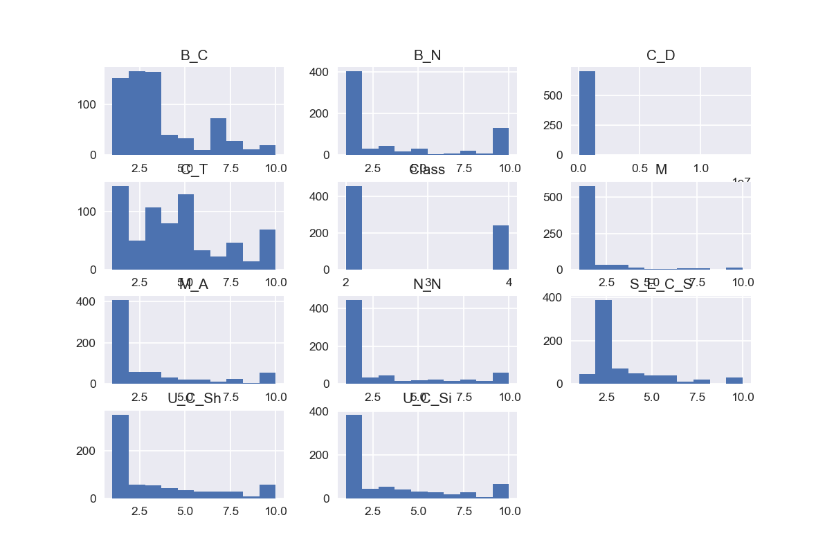
# 直方图
breast_cancer_data.hist()
pyplot.show()
In [19]:
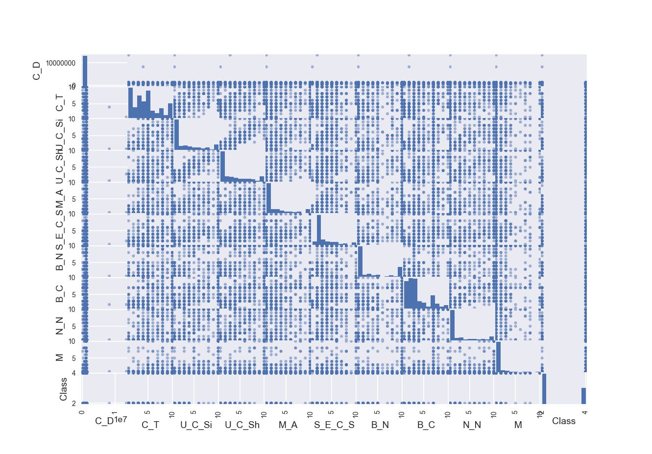
# 散点矩阵图
scatter_matrix(breast_cancer_data)
pyplot.show()
4.1分离数据集
In [52]:
# 分离数据集
array = breast_cancer_data.values
X = array[:, 1:9] # C_D为编号,与Y无相关性,过滤掉
Y = array[:, 10]


validation_size = 0.2
seed = 7
X_train, X_validation, Y_train, Y_validation = train_test_split(X, Y, test_size=validation_size, random_state=seed)
4.2评估算法
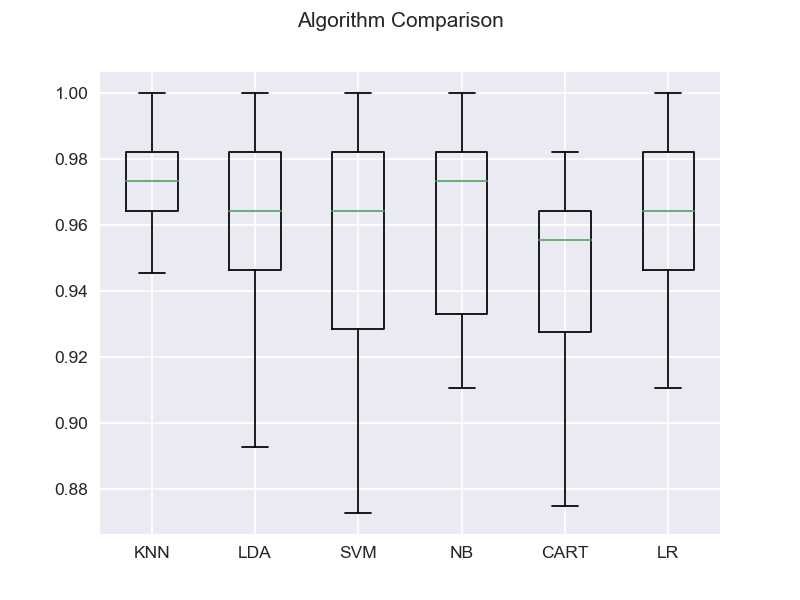
In [55]:
# 算法审查
models = {}
models['LR'] = LogisticRegression()
models['LDA'] = LinearDiscriminantAnalysis()
models['KNN'] = KNeighborsClassifier()
models['CART'] = DecisionTreeClassifier()
models['NB'] = GaussianNB()
models['SVM'] = SVC()

num_folds = 10
seed = 7
kfold = KFold(n_splits=num_folds, random_state=seed)
# 评估算法
results = []
for name in models:
    result = cross_val_score(models[name], X_train, Y_train, cv=kfold, scoring='accuracy')
    results.append(result)
    msg = '%s: %.3f (%.3f)' % (name, result.mean(), result.std())
    print(msg)

# 图表显示
fig = pyplot.figure()
fig.suptitle('Algorithm Comparison')
ax = fig.add_subplot(111)
pyplot.boxplot(results)
ax.set_xticklabels(models.keys())
pyplot.show()
In [75]:
#使用评估数据集评估算法
knn = KNeighborsClassifier()
knn.fit(X=X_train, y=Y_train)
predictions = knn.predict(X_validation)
print(accuracy_score(Y_validation, predictions))
print(confusion_matrix(Y_validation, predictions))
print(classification_report(Y_validation, predictions))