【SciKit-Learn学习笔记】3：线性回归测算波士顿房价,Logistic回归预测乳腺癌

版权声明：本文为博主原创学习笔记，如需转载请注明来源。 https://blog.csdn.net/SHU15121856/article/details/84310141

学习《scikit-learn机器学习》时的一些实践。

---

线性回归

这部分和第一篇笔记"绘制随机波动样本的学习曲线 "部分基本类似。线性回归里可以加入多项式特征，以对模型做增强。

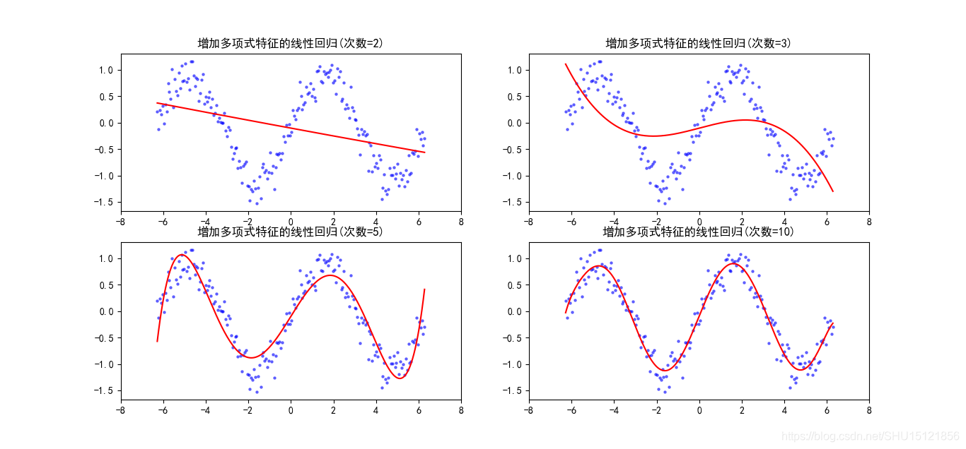
线性回归增加多项式特征,拟合sin函数

import numpy as np
import matplotlib.pyplot as plt
from sklearn.linear_model import LinearRegression
from sklearn.preprocessing import PolynomialFeatures
from sklearn.pipeline import Pipeline
from sklearn.metrics import mean_squared_error  # MSE损失
from matplotlib.figure import SubplotParams

# 使matplotlib正常显示负号
plt.rcParams['axes.unicode_minus'] = False

# 200个从-2pi到2pi的正弦函数样本点,上下波动0.1
n_dots = 200
X = np.linspace(-2 * np.pi, 2 * np.pi, n_dots)
y = np.sin(X) + 0.2 * np.random.randn(n_dots) - 0.1
X = X.reshape(-1, 1)
y = y.reshape(-1, 1)


# 多项式回归模型
def polynomial_model(degree=1):
    # 多项式模型,指定多项式的次数和是否使用偏置(常数项)
    polynomial_features = PolynomialFeatures(degree=degree, include_bias=False)
    # 线性回归模型,指定对每个特征归一化到(0,1)
    # (归一化只能提示算法收敛速度,不提高准确性)
    liner_regression = LinearRegression(normalize=True)
    # 装入管道
    pipline = Pipeline([("多项式", polynomial_features), ("线性回归", liner_regression)])
    return pipline


if __name__ == '__main__':
    degrees = [2, 3, 5, 10]
    models = []
    for d in degrees:
        model = polynomial_model(degree=d)
        # 这里会依次调用管道里的fit和transform(或者fit_transform),最后一个只调用fit
        model.fit(X, y)
        train_score = model.score(X, y)  # R2得分
        mse = mean_squared_error(y, model.predict(X))  # MSE损失
        print("degree:{}\tscore:{}\tmse loss:{}".format(d, train_score, mse))
        models.append({"model": model, "degree": d})  # 训练好的模型保存下来

    # 绘制不同degree的拟合结果,SubplotParams用于为子图设置统一参数,这里不用
    # plt.figure(figsize=(12, 6), dpi=200, subplotpars=SubplotParams(hspace=3.0))
    # fig, axes = plt.subplots(2, 2)
    for i, mod in enumerate(models):
        fig = plt.subplot(2, 2, i + 1)
        plt.xlim(-8, 8)
        plt.title("增加多项式特征的线性回归(次数={})".format(mod["degree"]))
        plt.scatter(X, y, s=5, c='b', alpha=0.5)
        plt.plot(X, mod["model"].predict(X), 'r-')
    # fig.tight_layout()
    plt.show()

运行结果：

degree:2	score:0.13584632282895104	mse loss:0.4661817984705142
degree:3	score:0.2876206298259192	mse loss:0.3843046725996981
degree:5	score:0.8483945839508078	mse loss:0.08178601489384577
degree:10	score:0.9330965409663139	mse loss:0.036092162401397294

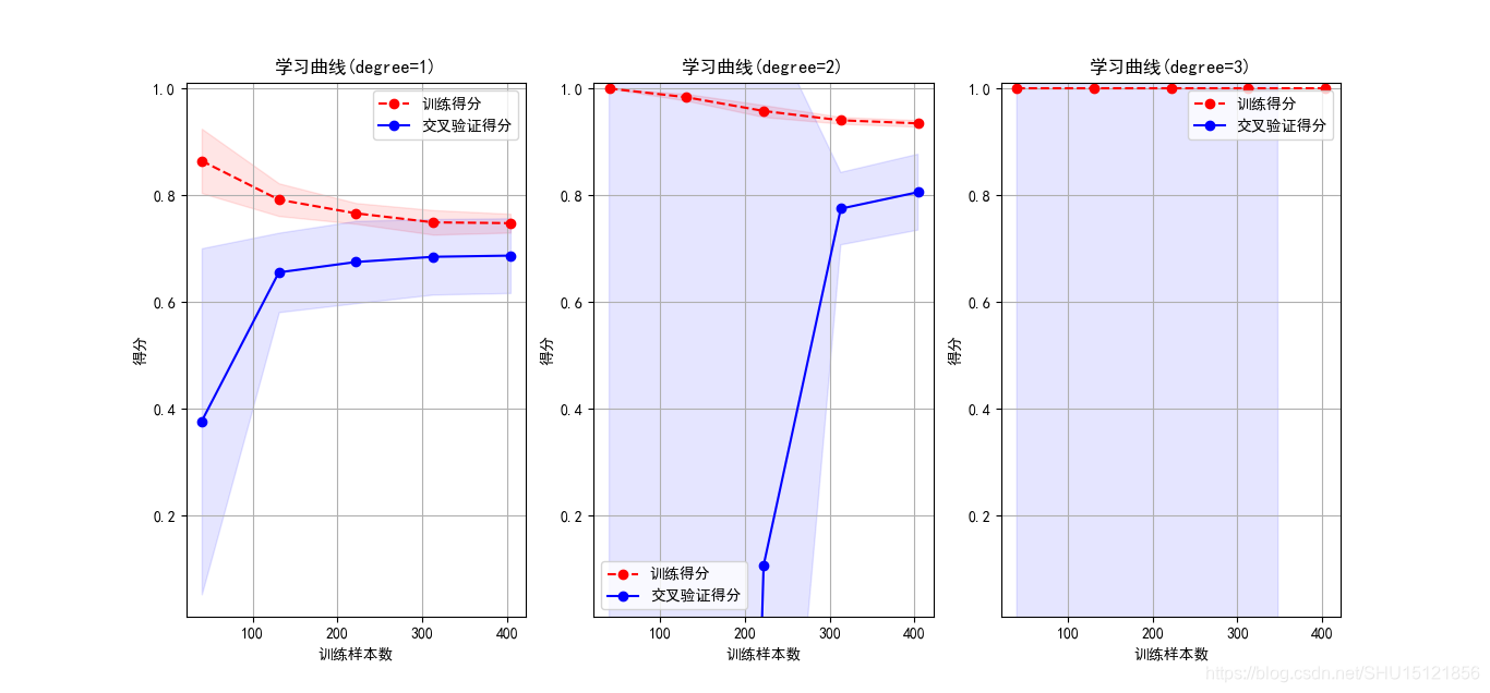
测算波士顿房价数据

在这个数据集上能更明显的看出第一篇里学的欠拟合和过拟合时候的学习曲线特征。

from sklearn.datasets import load_boston
from sklearn.model_selection import train_test_split
import time
from z5.liner_fit_sin import polynomial_model
from z3.learning_curve import plot_learning_curve
from sklearn.model_selection import ShuffleSplit
from matplotlib import pyplot as plt

# 读取boston房价数据集,并划分为训练集和测试集
boston = load_boston()
X = boston.data  # shape=(506,13)
y = boston.target  # shape=(506,)
X_train, X_test, y_train, y_test = train_test_split(X, y, test_size=0.2, random_state=3)

# 使用前面写的增加了多项式特征的线性回归模型
model = polynomial_model(degree=2)  # 改成3时验证集上得分:-104.825038,说明过拟合
start = time.clock()  # 计时:训练和测试打分的用时
model.fit(X_train, y_train)
train_score = model.score(X_train, y_train)
cv_score = model.score(X_test, y_test)
end = time.clock()
print("用时:{0:.6f},训练集上得分:{1:.6f},验证集上得分:{2:.6f}".format(end - start, train_score, cv_score))

# 绘制学习曲线
cv = ShuffleSplit(n_splits=10, test_size=0.2, random_state=0)
plt.figure(figsize=(18, 4), dpi=100)
org_title = "学习曲线(degree={})"
degrees = (1, 2, 3)

for i in range(len(degrees)):
    plt.subplot(1, 3, i + 1)
    plt = plot_learning_curve(polynomial_model(degrees[i]), org_title.format(degrees[i]), X, y, ylim=(0.01, 1.01),
                              cv=cv)
plt.show()

运行结果：

用时:0.027985,训练集上得分:0.930547,验证集上得分:0.860465

Logistic回归预测乳腺癌数据

Logistic回归也可以加多项式特征。

不带多项式特征的

注意，在计算ACC时书上作者的做法是错的，这里已经改正。

from sklearn.datasets import load_breast_cancer
from sklearn.model_selection import train_test_split
import numpy as np
from sklearn.linear_model import LogisticRegression
from sklearn.preprocessing import PolynomialFeatures
from sklearn.pipeline import Pipeline
import time
from z3.learning_curve import plot_learning_curve
from sklearn.model_selection import ShuffleSplit
from matplotlib import pyplot as plt

'''
logistic回归:乳腺癌数据
'''

# 读取和划分数据
cancer = load_breast_cancer()
X = cancer.data
y = cancer.target
print("X的shape={},正样本数:{},负样本数:{}".format(X.shape, y[y == 1].shape[0], y[y == 0].shape[0]))
X_train, X_test, y_train, y_test = train_test_split(X, y, test_size=0.2)

# 训练模型
model = LogisticRegression()
model.fit(X_train, y_train)

# 查看模型得分
train_score = model.score(X_train, y_train)
test_score = model.score(X_test, y_test)
print("训练集得分:{trs:.6f},测试集得分:{tss:.6f}".format(trs=train_score, tss=test_score))

# 对测试集做预测
y_pred = model.predict(X_test)
# 这里作者书上有重大失误.正确的是这样:np.equal可以比较两个数组中的每一项,返回True/False数组
# 然后使用np.count_nonzero()统计其中True的数目,也就是预测正确的样本数
print("ACC:{}/{}".format(np.count_nonzero(np.equal(y_pred, y_test)), y_test.shape[0]))

# 找出预测概率低于0.9的样本:概率和为1,所以两个概率都>0.1时预测概率低于0.9
# 返回样本被预测为各类的概率
y_pred_proba = model.predict_proba(X_test)
# 类别号是0和1,这里得到的第一列应是预测为0的概率,第二列是预测为1的概率,这里用断言确保一下
assert y_pred[0] == (0 if y_pred_proba[0, 0] > y_pred_proba[0, 1] else 1)
# 全部样本中,预测为阴性的p>0.1的部分
y_pp_big = y_pred_proba[y_pred_proba[:, 0] > 0.1]
# 在这个基础上,找其预测为阳性的p>0.1的部分
y_pp_big = y_pp_big[y_pp_big[:, 1] > 0.1]
print(y_pp_big.shape)

运行结果：

X的shape=(569, 30),正样本数:357,负样本数:212
训练集得分:0.962637,测试集得分:0.921053
ACC:105/114
(16, 2)

在前面的基础上添加多项式特征和L1正则化项

因为误差等值线和L1等值线相切的点在坐标轴上，所以L1范数正则化项解决过拟合的措施本质上是在减少特征的数量，即某些参数（在这里是多项式特征的系数）会减小到0。

L2范数的等值线是一个圆，所以和模型误差相切的点一般不在坐标轴上，其正则化项防止过拟合的措施实际上是让模型参数都尽可能小，都做出贡献，但不会小到0。

# 用pipeline为logistic回归模型增加多项式特征
def polynomial_model(degree=2, **kwargs):
    polynomial_features = PolynomialFeatures(degree=degree, include_bias=False)
    logistic_regression = LogisticRegression(**kwargs)
    pipeline = Pipeline([("多项式特征", polynomial_features), ("logistic回归", logistic_regression)])
    return pipeline


# 增加多项式特征后的模型
# 这里使用L1范数做正则项,实现参数稀疏化(让某些参数减少到0)从而留下对模型有帮助的特征
model = polynomial_model(degree=2, penalty='l1')
start = time.clock()  # 计时:训练和测试用时
model.fit(X_train, y_train)
train_score = model.score(X_train, y_train)
test_score = model.score(X_test, y_test)
end = time.clock()
print("用时:{0:.6f},训练集上得分:{1:.6f},测试集上得分:{2:.6f}".format(end - start, train_score, test_score))

# 观察一下有多少特征没有因L1范数正则化项而被丢弃(减小到0)
# 从管道中取出logistic回归的estimator,使用加入管道时给出的名字
logistic_regression = model.named_steps["logistic回归"]
# coef_属性里保存的就是模型参数的值
print("参数shape:{},其中非0项数目:{}".format(logistic_regression.coef_.shape, np.count_nonzero(logistic_regression.coef_)))

运行结果：

用时:0.237963,训练集上得分:1.000000,测试集上得分:0.947368
参数shape:(1, 495),其中非0项数目:88

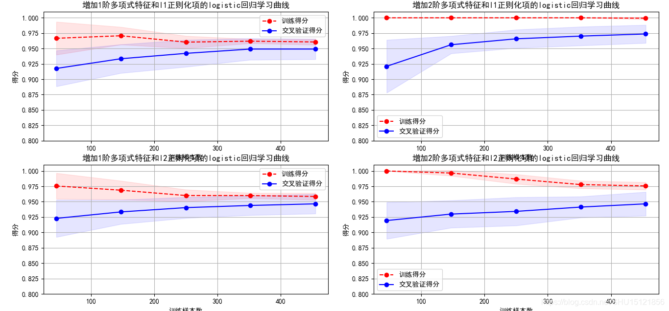
在前面的基础上比较使用L1和L2范数作为正则化项的学习曲线

# 绘制新模型的学习曲线
cv = ShuffleSplit(n_splits=10, test_size=0.2, random_state=0)
org_titlt = "增加{}阶多项式特征和{}正则化项的logistic回归学习曲线"
degrees = [1, 2]
penaltys = ["l1", "l2"]
fig = plt.figure(figsize=(12, 10), dpi=100)
for p in range(len(penaltys)):
    for i in range(len(degrees)):
        plt.subplot(len(penaltys), len(degrees), p * len(degrees) + i + 1)
        plt = plot_learning_curve(polynomial_model(degree=degrees[i], penalty=penaltys[p]),
                                  org_titlt.format(degrees[i], penaltys[p]), X, y, ylim=(0.8, 1.01), cv=cv)
fig.tight_layout()
plt.show()

运行结果：