Part 1: 构建神经网络

欢迎来到本周的第一个作业，这个作业我们将利用numpy实现你的第一个循环神经网络。

循环神经网络(Recurrent Neural Networks: RNN) 因为有”记忆”，所以在自然语言处理(Natural Language Processing) 和其他序列化任务中非常有效。RNN每次读取序列中的一个输入 $x^{<t>}$ (比如一个单词), 通过激活函数记住一些信息和上下文，然后传递到下一个实践部。这使得单向RNN可以携带信息想前传播，而双向RNN更是可以携带过去的和未来的上下文信息。

符号说明

上标 $^{[l]}$ 表示第l层
上标 $^{(i)}$ 表示第i个样本
上标 $^{<t>}$ 表示输入x在第t个时间步上的值
下标 $_i$ 表示一个向量的第i个维度
$T_x$ 和 $T_y$ 分别表示输入和输出的时间步数

导包

import numpy as np
from rnn_utils import *

下面是 rnn_utils 中包含的程序：

import numpy as np

def softmax(x):
    e_x = np.exp(x - np.max(x))
    return e_x / e_x.sum(axis=0)


def sigmoid(x):
    return 1 / (1 + np.exp(-x))


def initialize_adam(parameters) :
    """
    Initializes v and s as two python dictionaries with:
                - keys: "dW1", "db1", ..., "dWL", "dbL" 
                - values: numpy arrays of zeros of the same shape as the corresponding gradients/parameters.

    Arguments:
    parameters -- python dictionary containing your parameters.
                    parameters["W" + str(l)] = Wl
                    parameters["b" + str(l)] = bl

    Returns: 
    v -- python dictionary that will contain the exponentially weighted average of the gradient.
                    v["dW" + str(l)] = ...
                    v["db" + str(l)] = ...
    s -- python dictionary that will contain the exponentially weighted average of the squared gradient.
                    s["dW" + str(l)] = ...
                    s["db" + str(l)] = ...

    """

    L = len(parameters) // 2 # number of layers in the neural networks
    v = {}
    s = {}

    # Initialize v, s. Input: "parameters". Outputs: "v, s".
    for l in range(L):
    ### START CODE HERE ### (approx. 4 lines)
        v["dW" + str(l+1)] = np.zeros(parameters["W" + str(l+1)].shape)
        v["db" + str(l+1)] = np.zeros(parameters["b" + str(l+1)].shape)
        s["dW" + str(l+1)] = np.zeros(parameters["W" + str(l+1)].shape)
        s["db" + str(l+1)] = np.zeros(parameters["b" + str(l+1)].shape)
    ### END CODE HERE ###

    return v, s


def update_parameters_with_adam(parameters, grads, v, s, t, learning_rate = 0.01,
                                beta1 = 0.9, beta2 = 0.999,  epsilon = 1e-8):
    """
    Update parameters using Adam

    Arguments:
    parameters -- python dictionary containing your parameters:
                    parameters['W' + str(l)] = Wl
                    parameters['b' + str(l)] = bl
    grads -- python dictionary containing your gradients for each parameters:
                    grads['dW' + str(l)] = dWl
                    grads['db' + str(l)] = dbl
    v -- Adam variable, moving average of the first gradient, python dictionary
    s -- Adam variable, moving average of the squared gradient, python dictionary
    learning_rate -- the learning rate, scalar.
    beta1 -- Exponential decay hyperparameter for the first moment estimates 
    beta2 -- Exponential decay hyperparameter for the second moment estimates 
    epsilon -- hyperparameter preventing division by zero in Adam updates

    Returns:
    parameters -- python dictionary containing your updated parameters 
    v -- Adam variable, moving average of the first gradient, python dictionary
    s -- Adam variable, moving average of the squared gradient, python dictionary
    """

    L = len(parameters) // 2                 # number of layers in the neural networks
    v_corrected = {}                         # Initializing first moment estimate, python dictionary
    s_corrected = {}                         # Initializing second moment estimate, python dictionary

    # Perform Adam update on all parameters
    for l in range(L):
        # Moving average of the gradients. Inputs: "v, grads, beta1". Output: "v".
        ### START CODE HERE ### (approx. 2 lines)
        v["dW" + str(l+1)] = beta1 * v["dW" + str(l+1)] + (1 - beta1) * grads["dW" + str(l+1)] 
        v["db" + str(l+1)] = beta1 * v["db" + str(l+1)] + (1 - beta1) * grads["db" + str(l+1)] 
        ### END CODE HERE ###

        # Compute bias-corrected first moment estimate. Inputs: "v, beta1, t". Output: "v_corrected".
        ### START CODE HERE ### (approx. 2 lines)
        v_corrected["dW" + str(l+1)] = v["dW" + str(l+1)] / (1 - beta1**t)
        v_corrected["db" + str(l+1)] = v["db" + str(l+1)] / (1 - beta1**t)
        ### END CODE HERE ###

        # Moving average of the squared gradients. Inputs: "s, grads, beta2". Output: "s".
        ### START CODE HERE ### (approx. 2 lines)
        s["dW" + str(l+1)] = beta2 * s["dW" + str(l+1)] + (1 - beta2) * (grads["dW" + str(l+1)] ** 2)
        s["db" + str(l+1)] = beta2 * s["db" + str(l+1)] + (1 - beta2) * (grads["db" + str(l+1)] ** 2)
        ### END CODE HERE ###

        # Compute bias-corrected second raw moment estimate. Inputs: "s, beta2, t". Output: "s_corrected".
        ### START CODE HERE ### (approx. 2 lines)
        s_corrected["dW" + str(l+1)] = s["dW" + str(l+1)] / (1 - beta2 ** t)
        s_corrected["db" + str(l+1)] = s["db" + str(l+1)] / (1 - beta2 ** t)
        ### END CODE HERE ###

        # Update parameters. Inputs: "parameters, learning_rate, v_corrected, s_corrected, epsilon". Output: "parameters".
        ### START CODE HERE ### (approx. 2 lines)
        parameters["W" + str(l+1)] = parameters["W" + str(l+1)] - learning_rate * v_corrected["dW" + str(l+1)] / np.sqrt(s_corrected["dW" + str(l+1)] + epsilon)
        parameters["b" + str(l+1)] = parameters["b" + str(l+1)] - learning_rate * v_corrected["db" + str(l+1)] / np.sqrt(s_corrected["db" + str(l+1)] + epsilon)
        ### END CODE HERE ###

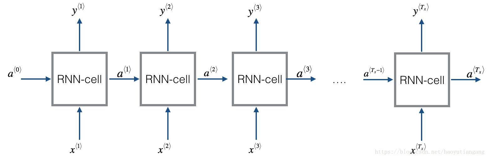
    return parameters, v, s

1 基本循环神经网络的前向传播

基本的RNN结构如下：(这里Tx = Ty)

实现循环神经网络

实现 RNN 单时间步运算
按时间循环Tx的每个时间步运算

1.1 RNN 单元

一个循环神经网络可以看成是单个RNN单元的重复。首先我们将实现一个单时间步的RNN单元的计算，下图描述了单步RNN 的操作。

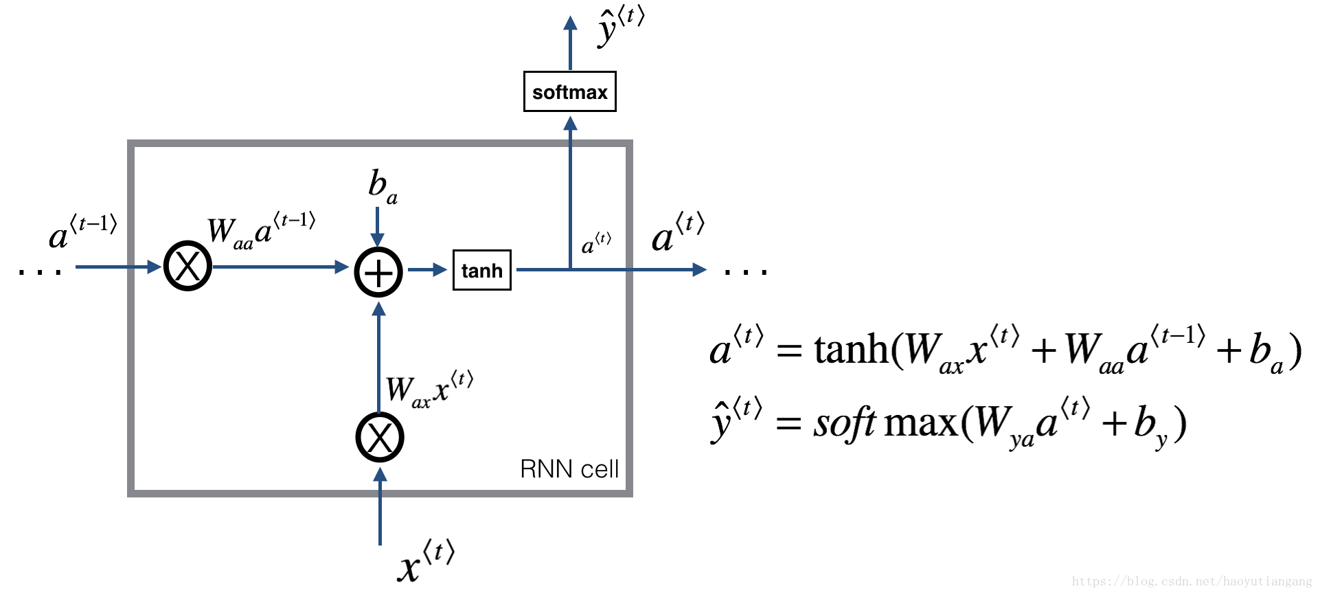
练习：实现上图描述的单步RNN单元

利用tanh激活函数计算隐藏层的状态
$a^{⟨ t ⟩} = \tanh (W_{a a} a^{⟨ t - 1 ⟩} + W_{a x} x^{⟨ t ⟩} + b_{a})$ $a^{\langle t \rangle} = \tanh(W_{aa} a^{\langle t-1 \rangle} + W_{ax} x^{\langle t \rangle} + b_a)$
使用新的隐藏层状态 $a^{<t>}$ 计算预测值 $y_{hat}$ （已提供函数softmax）
${\hat{y}}^{⟨ t ⟩} = s o f t m a x (W_{y a} a^{⟨ t ⟩} + b_{y})$ $\hat{y}^{\langle t \rangle} = softmax(W_{ya} a^{\langle t \rangle} + b_y)$
在cache中存储参数
$(a^{⟨ t ⟩}, a^{⟨ t - 1 ⟩}, x^{⟨ t ⟩}, p a r a m e t e r s)$ $(a^{\langle t \rangle}, a^{\langle t-1 \rangle}, x^{\langle t \rangle}, parameters)$
返回 $a^{<t>}$ , $y^{<t>}$ 和 cache

我们的输入是m个向量。所以： $x^{<t>}$ 维度：( $n_x$ , m) ; $a^{<t>}$ 维度：( $n_a$ , m)

# GRADED FUNCTION: rnn_cell_forward

def rnn_cell_forward(xt, a_prev, parameters):
    """
    Implements a single forward step of the RNN-cell as described in Figure (2)

    Arguments:
    xt -- your input data at timestep "t", numpy array of shape (n_x, m).
    a_prev -- Hidden state at timestep "t-1", numpy array of shape (n_a, m)
    parameters -- python dictionary containing:
                        Wax -- Weight matrix multiplying the input, numpy array of shape (n_a, n_x)
                        Waa -- Weight matrix multiplying the hidden state, numpy array of shape (n_a, n_a)
                        Wya -- Weight matrix relating the hidden-state to the output, numpy array of shape (n_y, n_a)
                        ba --  Bias, numpy array of shape (n_a, 1)
                        by -- Bias relating the hidden-state to the output, numpy array of shape (n_y, 1)
    Returns:
    a_next -- next hidden state, of shape (n_a, m)
    yt_pred -- prediction at timestep "t", numpy array of shape (n_y, m)
    cache -- tuple of values needed for the backward pass, contains (a_next, a_prev, xt, parameters)
    """

    # Retrieve parameters from "parameters"
    Wax = parameters["Wax"]
    Waa = parameters["Waa"]
    Wya = parameters["Wya"]
    ba = parameters["ba"]
    by = parameters["by"]

    ### START CODE HERE ### (≈2 lines)
    # compute next activation state using the formula given above
    a_next = np.tanh(np.dot(Waa, a_prev) + np.dot(Wax, xt) + ba)
    # compute output of the current cell using the formula given above
    yt_pred = softmax(np.dot(Wya, a_next) + by) 
    ### END CODE HERE ###

    # store values you need for backward propagation in cache
    cache = (a_next, a_prev, xt, parameters)

    return a_next, yt_pred, cache

#########################################################

np.random.seed(1)
xt = np.random.randn(3,10)
a_prev = np.random.randn(5,10)
Waa = np.random.randn(5,5)
Wax = np.random.randn(5,3)
Wya = np.random.randn(2,5)
ba = np.random.randn(5,1)
by = np.random.randn(2,1)
parameters = {"Waa": Waa, "Wax": Wax, "Wya": Wya, "ba": ba, "by": by}

a_next, yt_pred, cache = rnn_cell_forward(xt, a_prev, parameters)
print("a_next[4] = ", a_next[4])
print("a_next.shape = ", a_next.shape)
print("yt_pred[1] =", yt_pred[1])
print("yt_pred.shape = ", yt_pred.shape)

# a_next[4] =  [ 0.59584544  0.18141802  0.61311866  0.99808218  0.85016201  # 0.99980978
#  -0.18887155  0.99815551  0.6531151   0.82872037]
# a_next.shape =  (5, 10)
# yt_pred[1] = [ 0.9888161   0.01682021  0.21140899  0.36817467  0.98988387  # 0.88945212
#   0.36920224  0.9966312   0.9982559   0.17746526]
# yt_pred.shape =  (2, 10)

期待输出

key	value
a_next[4]:	[ 0.59584544 0.18141802 0.61311866 0.99808218 0.85016201 0.99980978 -0.18887155 0.99815551 0.6531151 0.82872037]
a_next.shape:	(5, 10)
yt[1]:	[ 0.9888161 0.01682021 0.21140899 0.36817467 0.98988387 0.88945212 0.36920224 0.9966312 0.9982559 0.17746526]
yt.shape:	(2, 10)

1.2 RNN 前向传播

比如输入有10个时间步，则依次将单元RNN相连，每个单元的输入来自上层的 $a^{<t-1>}$ 和本层的 $x^{<t>}$ ，输出 $a^{<t>}$ 和 $y_{hat}^{<t>}$ 。

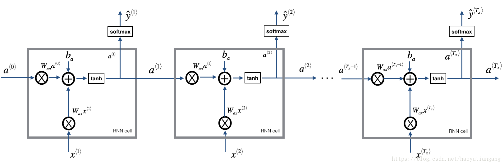
练习：实现上图描述的RNN 的前向传播

创建一个0值向量a, 用来存储RNN计算的所有隐藏状态
初始化”next”隐藏层状态 $a_0$
循环每个时间步，循环变量为t
- 执行rnn_cell_forward，升级”next”隐藏状态和缓存
- 存储”next”隐藏状态到a( $t^{th}$ 位置)
- 村塾预测输出y
- 将cache加到列表 caches 中
返回a, y 和caches

# GRADED FUNCTION: rnn_forward

def rnn_forward(x, a0, parameters):
    """
    Implement the forward propagation of the recurrent neural network described in Figure (3).

    Arguments:
    x -- Input data for every time-step, of shape (n_x, m, T_x).
    a0 -- Initial hidden state, of shape (n_a, m)
    parameters -- python dictionary containing:
                        Waa -- Weight matrix multiplying the hidden state, numpy array of shape (n_a, n_a)
                        Wax -- Weight matrix multiplying the input, numpy array of shape (n_a, n_x)
                        Wya -- Weight matrix relating the hidden-state to the output, numpy array of shape (n_y, n_a)
                        ba --  Bias numpy array of shape (n_a, 1)
                        by -- Bias relating the hidden-state to the output, numpy array of shape (n_y, 1)

    Returns:
    a -- Hidden states for every time-step, numpy array of shape (n_a, m, T_x)
    y_pred -- Predictions for every time-step, numpy array of shape (n_y, m, T_x)
    caches -- tuple of values needed for the backward pass, contains (list of caches, x)
    """

    # Initialize "caches" which will contain the list of all caches
    caches = []

    # Retrieve dimensions from shapes of x and parameters["Wya"]
    n_x, m, T_x = x.shape
    n_y, n_a = parameters["Wya"].shape

    ### START CODE HERE ###

    # initialize "a" and "y" with zeros (≈2 lines)
    a = np.zeros((n_a, m, T_x))
    y_pred = np.zeros((n_y, m, T_x))

    # Initialize a_next (≈1 line)
    a_next = a0

    # loop over all time-steps
    for t in range(T_x):
        # Update next hidden state, compute the prediction, get the cache (≈1 line)
        a_next, yt_pred, cache = rnn_cell_forward(x[:, :, t], a_next, parameters)
        # Save the value of the new "next" hidden state in a (≈1 line)
        a[:,:,t] = a_next
        # Save the value of the prediction in y (≈1 line)
        y_pred[:,:,t] = yt_pred
        # Append "cache" to "caches" (≈1 line)
        caches.append(cache)

    ### END CODE HERE ###

    # store values needed for backward propagation in cache
    caches = (caches, x)

    return a, y_pred, caches

################################################3

np.random.seed(1)
x = np.random.randn(3,10,4)
a0 = np.random.randn(5,10)
Waa = np.random.randn(5,5)
Wax = np.random.randn(5,3)
Wya = np.random.randn(2,5)
ba = np.random.randn(5,1)
by = np.random.randn(2,1)
parameters = {"Waa": Waa, "Wax": Wax, "Wya": Wya, "ba": ba, "by": by}

a, y_pred, caches = rnn_forward(x, a0, parameters)
print("a[4][1] = ", a[4][1])
print("a.shape = ", a.shape)
print("y_pred[1][3] =", y_pred[1][3])
print("y_pred.shape = ", y_pred.shape)
print("caches[1][1][3] =", caches[1][1][3])
print("len(caches) = ", len(caches))

# a[4][1] =  [-0.99999375  0.77911235 -0.99861469 -0.99833267]
# a.shape =  (5, 10, 4)
# y_pred[1][3] = [ 0.79560373  0.86224861  0.11118257  0.81515947]
# y_pred.shape =  (2, 10, 4)
# caches[1][1][3] = [-1.1425182  -0.34934272 -0.20889423  0.58662319]
# len(caches) =  2

期待输出

key	value
a[4][1]:	[-0.99999375 0.77911235 -0.99861469 -0.99833267]
a.shape:	(5, 10, 4)
y[1][3]:	[ 0.79560373 0.86224861 0.11118257 0.81515947]
y.shape:	(2, 10, 4)
cache[1][1][3]:	[-1.1425182 -0.34934272 -0.20889423 0.58662319]
len(cache):	2

恭喜！你已经建立了一个循环审计网络的前向传播函数。在一些情况下你的程序运行良好。但是存在梯度消失的问题。如果能在近距离评估每个 $y_{hat}$ 的话程序将会执行的更好。

在下个部分，我们将建立一个更复杂的LSTM模型，它可以有效的定位梯度消失的问题。LSTM 将会记住一个信息片段并保持许多步的向前传播。

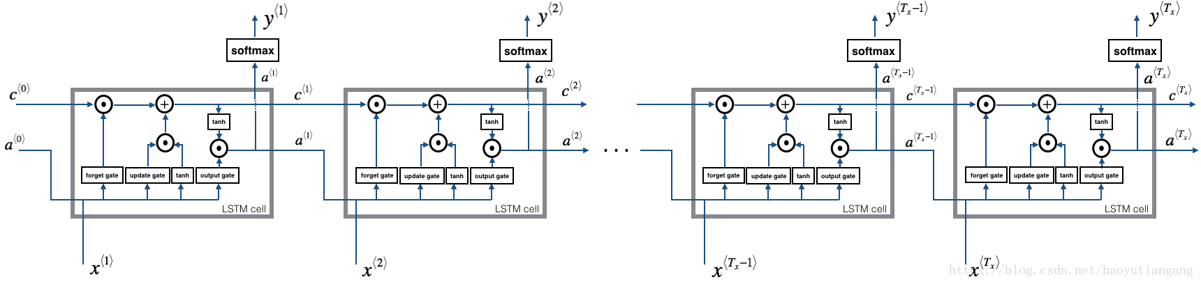
2 长短时记忆网络(Long Short Term Memory (LSTM))

下图描述了LSTM单元的操作

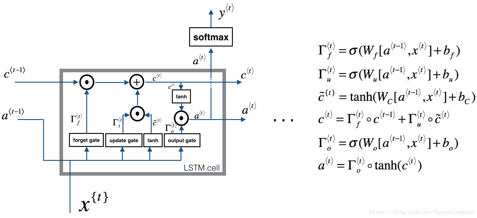
与上文类似，我们将先实现单步的LSTM 单元，然后再循环各个时间步。

2.0 关于门

2.0.1 遗忘门

假设我们正在阅读一段文字中的单词，并且希望使用LSTM来跟踪语法结构，例如主语是单数还是复数。如果主语从单个单词变成复数单词，我们需要找到一种方法来摆脱先前存储的单数/复数状态的记忆值。

在LSTM中，遗忘门让我们做到这一点：

Γ_{f}^{⟨ t ⟩} = σ (W_{f} [a^{⟨ t - 1 ⟩}, x^{⟨ t ⟩}] + b_{f})

$\Gamma_f^{\langle t \rangle} = \sigma(W_f[a^{\langle t-1 \rangle}, x^{\langle t \rangle}] + b_f)$

这里， $W_f$ 是管理遗忘门行为的权重。我们连接 $[a^{⟨t-1⟩}，x^{⟨t⟩}]$ 并乘以Wf。上面的等式产生了一个向量 $Γ_f^{⟨t⟩}$ ，其值介于0和1之间。这个遗忘的门向量的每个元素都乘以前一个单元状态 $c^{⟨t-1⟩}$ 。因此，如果 $Γ_f^{⟨t⟩}$ 的值之一是0（或接近于0），那么它意味着LSTM应该删除 $c^{⟨t-1⟩}$ 的相应分量中的那条信息（例如单个主体）。如果其中一个值为1，则它将保留该信息。

2.0.2 更新门

一旦我们忘记所讨论的主题是单数的，我们需要找到一种方法来更新它，以反映新主题现在是复数。

这是更新门的公式：

Γ_{u}^{⟨ t ⟩} = σ (W_{u} [a^{⟨ t - 1 ⟩}, x^{{t}}] + b_{u})

$\Gamma_u^{\langle t \rangle} = \sigma(W_u[a^{\langle t-1 \rangle}, x^{\{t\}}] + b_u)$
类似于遗忘门，这里

Γ_{u}^{⟨ t ⟩}

$Γ_u^{⟨t⟩}$ 也是一个介于0和1之间的值的向量。为了计算

c^{< t >}

$c^{<t>}$ ，它将与

c ̃^{⟨ t ⟩}

$c̃ ^{⟨t⟩}$ 逐元相乘。

2.0.3 更新单元值

为了更新新单元，我们需要创建一个新的数字向量，可以更新到元旦的单元状态中。公式如下:

{\tilde{c}}^{⟨ t ⟩} = \tanh (W_{c} [a^{⟨ t - 1 ⟩}, x^{⟨ t ⟩}] + b_{c})

$\tilde{c}^{\langle t \rangle} = \tanh(W_c[a^{\langle t-1 \rangle}, x^{\langle t \rangle}] + b_c)$
最后，新单元为：

c^{⟨ t ⟩} = Γ_{f}^{⟨ t ⟩} * c^{⟨ t - 1 ⟩} + Γ_{u}^{⟨ t ⟩} * {\tilde{c}}^{⟨ t ⟩}

$c^{\langle t \rangle} = \Gamma_f^{\langle t \rangle}* c^{\langle t-1 \rangle} + \Gamma_u^{\langle t \rangle} *\tilde{c}^{\langle t \rangle}$

2.0.4 输出门

为了决定输出，我们将使用以下两个公式：

Γ_{o}^{⟨ t ⟩} = σ (W_{o} [a^{⟨ t - 1 ⟩}, x^{⟨ t ⟩}] + b_{o})

$\Gamma_o^{\langle t \rangle}= \sigma(W_o[a^{\langle t-1 \rangle}, x^{\langle t \rangle}] + b_o)$

a^{⟨ t ⟩} = Γ_{o}^{⟨ t ⟩} * \tanh (c^{⟨ t ⟩})

$a^{\langle t \rangle} = \Gamma_o^{\langle t \rangle}* \tanh(c^{\langle t \rangle})$
第一个公式利用sigmoid函数决定输出，第二个公式将之前的状态乘以tanh函数。

2.1 LSTM 单元

练习：实现上文描述的LSTM单元
1. 连接 $a^{<t-1>}$ , $x^{<t>}$ 为一个矩阵

c o n c a t = [\begin{matrix} a^{⟨ t - 1 ⟩} \\ x^{⟨ t ⟩} \end{matrix}]

$concat = \begin{bmatrix} a^{\langle t-1 \rangle} \\ x^{\langle t \rangle} \end{bmatrix}$
2. 计算上文各个公式，可以使用已提供的sigmoid函数和np.tanh函数
3. 计算预测的输出y，可以使用已提供的softmax函数

# GRADED FUNCTION: lstm_cell_forward

def lstm_cell_forward(xt, a_prev, c_prev, parameters):
    """
    Implement a single forward step of the LSTM-cell as described in Figure (4)

    Arguments:
    xt -- your input data at timestep "t", numpy array of shape (n_x, m).
    a_prev -- Hidden state at timestep "t-1", numpy array of shape (n_a, m)
    c_prev -- Memory state at timestep "t-1", numpy array of shape (n_a, m)
    parameters -- python dictionary containing:
                        Wf -- Weight matrix of the forget gate, numpy array of shape (n_a, n_a + n_x)
                        bf -- Bias of the forget gate, numpy array of shape (n_a, 1)
                        Wi -- Weight matrix of the update gate, numpy array of shape (n_a, n_a + n_x)
                        bi -- Bias of the update gate, numpy array of shape (n_a, 1)
                        Wc -- Weight matrix of the first "tanh", numpy array of shape (n_a, n_a + n_x)
                        bc --  Bias of the first "tanh", numpy array of shape (n_a, 1)
                        Wo -- Weight matrix of the output gate, numpy array of shape (n_a, n_a + n_x)
                        bo --  Bias of the output gate, numpy array of shape (n_a, 1)
                        Wy -- Weight matrix relating the hidden-state to the output, numpy array of shape (n_y, n_a)
                        by -- Bias relating the hidden-state to the output, numpy array of shape (n_y, 1)

    Returns:
    a_next -- next hidden state, of shape (n_a, m)
    c_next -- next memory state, of shape (n_a, m)
    yt_pred -- prediction at timestep "t", numpy array of shape (n_y, m)
    cache -- tuple of values needed for the backward pass, contains (a_next, c_next, a_prev, c_prev, xt, parameters)

    Note: ft/it/ot stand for the forget/update/output gates, cct stands for the candidate value (c tilde),
          c stands for the memory value
    """

    # Retrieve parameters from "parameters"
    Wf = parameters["Wf"]
    bf = parameters["bf"]
    Wi = parameters["Wi"]
    bi = parameters["bi"]
    Wc = parameters["Wc"]
    bc = parameters["bc"]
    Wo = parameters["Wo"]
    bo = parameters["bo"]
    Wy = parameters["Wy"]
    by = parameters["by"]

    # Retrieve dimensions from shapes of xt and Wy
    n_x, m = xt.shape
    n_y, n_a = Wy.shape

    ### START CODE HERE ###
    # Concatenate a_prev and xt (≈3 lines)
    concat = np.zeros((n_x + n_a, m))
    concat[: n_a, :] = a_prev  
    concat[n_a :, :] = xt 

    # Compute values for ft, it, cct, c_next, ot, a_next using the formulas given figure (4) (≈6 lines)
    ft = sigmoid(np.dot(Wf, concat) + bf)
    it = sigmoid(np.dot(Wi, concat) + bi)
    cct = np.tanh(np.dot(Wc, concat) + bc)
    c_next = ft*c_prev + it*cct
    ot = sigmoid(np.dot(Wo, concat) + bo)
    a_next = ot*np.tanh(c_next)

    # Compute prediction of the LSTM cell (≈1 line)
    yt_pred = softmax(np.dot(Wy, a_next) + by)
    ### END CODE HERE ###

    # store values needed for backward propagation in cache
    cache = (a_next, c_next, a_prev, c_prev, ft, it, cct, ot, xt, parameters)

    return a_next, c_next, yt_pred, cache

########################################################3

np.random.seed(1)
xt = np.random.randn(3,10)
a_prev = np.random.randn(5,10)
c_prev = np.random.randn(5,10)
Wf = np.random.randn(5, 5+3)
bf = np.random.randn(5,1)
Wi = np.random.randn(5, 5+3)
bi = np.random.randn(5,1)
Wo = np.random.randn(5, 5+3)
bo = np.random.randn(5,1)
Wc = np.random.randn(5, 5+3)
bc = np.random.randn(5,1)
Wy = np.random.randn(2,5)
by = np.random.randn(2,1)

parameters = {"Wf": Wf, "Wi": Wi, "Wo": Wo, "Wc": Wc, "Wy": Wy, "bf": bf, "bi": bi, "bo": bo, "bc": bc, "by": by}

a_next, c_next, yt, cache = lstm_cell_forward(xt, a_prev, c_prev, parameters)
print("a_next[4] = ", a_next[4])
print("a_next.shape = ", c_next.shape)
print("c_next[2] = ", c_next[2])
print("c_next.shape = ", c_next.shape)
print("yt[1] =", yt[1])
print("yt.shape = ", yt.shape)
print("cache[1][3] =", cache[1][3])
print("len(cache) = ", len(cache))

# a_next[4] =  [-0.66408471  0.0036921   0.02088357  0.22834167 -0.85575339  # 0.00138482
#   0.76566531  0.34631421 -0.00215674  0.43827275]
# a_next.shape =  (5, 10)
# c_next[2] =  [ 0.63267805  1.00570849  0.35504474  0.20690913 -1.64566718  # 0.11832942
#   0.76449811 -0.0981561  -0.74348425 -0.26810932]
# c_next.shape =  (5, 10)
# yt[1] = [ 0.79913913  0.15986619  0.22412122  0.15606108  0.97057211  # 0.31146381
#   0.00943007  0.12666353  0.39380172  0.07828381]
# yt.shape =  (2, 10)
# cache[1][3] = [-0.16263996  1.03729328  0.72938082 -0.54101719  0.02752074 # -0.30821874
#   0.07651101 -1.03752894  1.41219977 -0.37647422]
# len(cache) =  10

期待的输出

key	value
a_next[4]:	[-0.66408471 0.0036921 0.02088357 0.22834167 -0.85575339 0.00138482 0.76566531 0.34631421 -0.00215674 0.43827275]
a_next.shape:	(5, 10)
c_next[2]:	[ 0.63267805 1.00570849 0.35504474 0.20690913 -1.64566718 0.11832942 0.76449811 -0.0981561 -0.74348425 -0.26810932]
c_next.shape:	(5, 10)
yt[1]:	[ 0.79913913 0.15986619 0.22412122 0.15606108 0.97057211 0.31146381 0.00943007 0.12666353 0.39380172 0.07828381]
yt.shape:	(2, 10)
cache[1][3]:	[-0.16263996 1.03729328 0.72938082 -0.54101719 0.02752074 -0.30821874 0.07651101 -1.03752894 1.41219977 -0.37647422]
len(cache):	10

2.2 LSTM的前向传播

现在你已经实现了单步的LSTM，下面可以迭代循环了

练习：实现lstm_forward()

$c^{<0>}$ 是0值初始化向量

# GRADED FUNCTION: lstm_forward

def lstm_forward(x, a0, parameters):
    """
    Implement the forward propagation of the recurrent neural network using an LSTM-cell described in Figure (3).

    Arguments:
    x -- Input data for every time-step, of shape (n_x, m, T_x).
    a0 -- Initial hidden state, of shape (n_a, m)
    parameters -- python dictionary containing:
                        Wf -- Weight matrix of the forget gate, numpy array of shape (n_a, n_a + n_x)
                        bf -- Bias of the forget gate, numpy array of shape (n_a, 1)
                        Wi -- Weight matrix of the update gate, numpy array of shape (n_a, n_a + n_x)
                        bi -- Bias of the update gate, numpy array of shape (n_a, 1)
                        Wc -- Weight matrix of the first "tanh", numpy array of shape (n_a, n_a + n_x)
                        bc -- Bias of the first "tanh", numpy array of shape (n_a, 1)
                        Wo -- Weight matrix of the output gate, numpy array of shape (n_a, n_a + n_x)
                        bo -- Bias of the output gate, numpy array of shape (n_a, 1)
                        Wy -- Weight matrix relating the hidden-state to the output, numpy array of shape (n_y, n_a)
                        by -- Bias relating the hidden-state to the output, numpy array of shape (n_y, 1)

    Returns:
    a -- Hidden states for every time-step, numpy array of shape (n_a, m, T_x)
    y -- Predictions for every time-step, numpy array of shape (n_y, m, T_x)
    caches -- tuple of values needed for the backward pass, contains (list of all the caches, x)
    """

    # Initialize "caches", which will track the list of all the caches
    caches = []

    ### START CODE HERE ###
    # Retrieve dimensions from shapes of x and parameters['Wy'] (≈2 lines)
    n_x, m, T_x = x.shape
    n_y, n_a = parameters['Wy'].shape

    # initialize "a", "c" and "y" with zeros (≈3 lines)
    a = np.zeros((n_a, m, T_x))
    c = np.zeros((n_a, m, T_x))
    y = np.zeros((n_y, m, T_x))

    # Initialize a_next and c_next (≈2 lines)
    a_next = a0
    c_next = np.zeros((n_a, m))

    # loop over all time-steps
    for t in range(T_x):
        # Update next hidden state, next memory state, compute the prediction, get the cache (≈1 line)
        a_next, c_next, yt, cache = lstm_cell_forward(x[:, :, t], a_next, c_next, parameters)
        # Save the value of the new "next" hidden state in a (≈1 line)
        a[:,:,t] = a_next
        # Save the value of the prediction in y (≈1 line)
        y[:,:,t] = yt
        # Save the value of the next cell state (≈1 line)
        c[:,:,t]  = c_next
        # Append the cache into caches (≈1 line)
        caches.append(cache)

    ### END CODE HERE ###

    # store values needed for backward propagation in cache
    caches = (caches, x)

    return a, y, c, caches

##########################################################

np.random.seed(1)
x = np.random.randn(3,10,7)
a0 = np.random.randn(5,10)
Wf = np.random.randn(5, 5+3)
bf = np.random.randn(5,1)
Wi = np.random.randn(5, 5+3)
bi = np.random.randn(5,1)
Wo = np.random.randn(5, 5+3)
bo = np.random.randn(5,1)
Wc = np.random.randn(5, 5+3)
bc = np.random.randn(5,1)
Wy = np.random.randn(2,5)
by = np.random.randn(2,1)

parameters = {"Wf": Wf, "Wi": Wi, "Wo": Wo, "Wc": Wc, "Wy": Wy, "bf": bf, "bi": bi, "bo": bo, "bc": bc, "by": by}

a, y, c, caches = lstm_forward(x, a0, parameters)
print("a[4][3][6] = ", a[4][3][6])
print("a.shape = ", a.shape)
print("y[1][4][3] =", y[1][4][3])
print("y.shape = ", y.shape)
print("caches[1][1[1]] =", caches[1][1][1])
print("c[1][2][1]", c[1][2][1])
print("len(caches) = ", len(caches))

# a[4][3][6] =  0.172117767533
# a.shape =  (5, 10, 7)
# y[1][4][3] = 0.95087346185
# y.shape =  (2, 10, 7)
# caches[1][1[1]] = [ 0.82797464  0.23009474  0.76201118 -0.22232814 # -0.20075807  0.18656139
#   0.41005165]
# c[1][2][1] -0.855544916718
# len(caches) =  2

期待的输出

key	value
a[4][3][6]	0.172117767533
a.shape	(5, 10, 7)
y[1][4][3]	0.95087346185
y.shape	(2, 10, 7)
caches[1][1][1]	[ 0.82797464 0.23009474 0.76201118 -0.22232814 -0.20075807 0.18656139 0.41005165]
c[1][2][1]	-0.855544916718
len(caches)	2

恭喜！你已经完成了基本RNN和LSTM的前向传播。使用深度学习框架的时候，只实现前向传播已经足够了。

下面反向传播的部分是可选的。

3 循环神经网络的反向传播 (可选)

在之前的课程中，你实现了一个简单的（完全连接的）神经网络，并使用反向传播来计算更新损失函数的梯度。同样，在递归神经网络中，您可以根据损失函数的梯度以更新参数。

3.1 基本 RNN 的反向传播

3.1.1 基本 RNN 单元的反向传播计算

t a n h^{'} (x) = 1 - t a n h^{2} (x)

$tanh'(x) = 1 - tanh^2(x)$
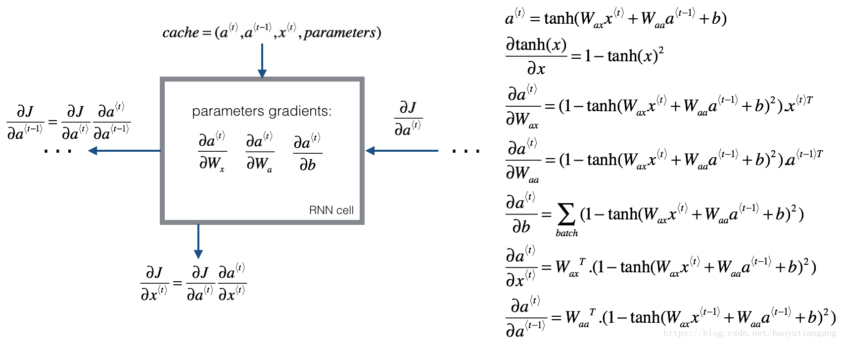
导数的矩阵维度与其原函数一致。

def rnn_cell_backward(da_next, cache):
    """
    Implements the backward pass for the RNN-cell (single time-step).

    Arguments:
    da_next -- Gradient of loss with respect to next hidden state
    cache -- python dictionary containing useful values (output of rnn_cell_forward())

    Returns:
    gradients -- python dictionary containing:
                        dx -- Gradients of input data, of shape (n_x, m)
                        da_prev -- Gradients of previous hidden state, of shape (n_a, m)
                        dWax -- Gradients of input-to-hidden weights, of shape (n_a, n_x)
                        dWaa -- Gradients of hidden-to-hidden weights, of shape (n_a, n_a)
                        dba -- Gradients of bias vector, of shape (n_a, 1)
    """

    # Retrieve values from cache
    (a_next, a_prev, xt, parameters) = cache

    # Retrieve values from parameters
    Wax = parameters["Wax"]
    Waa = parameters["Waa"]
    Wya = parameters["Wya"]
    ba = parameters["ba"]
    by = parameters["by"]

    ### START CODE HERE ###
    # compute the gradient of tanh with respect to a_next (≈1 line)
    # 根据上面提供的参数 da_next -- Gradient of loss with respect to next hidden state 
    # 以及提到的公式 tanh(u) = (1- tanh(u)**2)*du ，这里du 就是da_next、tanh(u)是a_next
    dtanh = (1-a_next**2)*da_next    # formula 1、2

    # compute the gradient of the loss with respect to Wax (≈2 lines)
    dxt = np.dot(Wax.T, dtanh)    # formula 6
    dWax = np.dot(dtanh, xt.T)    # formula 3

    # compute the gradient with respect to Waa (≈2 lines)
    da_prev = np.dot(Waa.T, dtanh)    # formula 7
    dWaa = np.dot(dtanh, a_prev.T)    # formula 4

    # compute the gradient with respect to b (≈1 line)
    dba = np.sum(dtanh, keepdims=True, axis=-1)    # formula 5

    ### END CODE HERE ###

    # Store the gradients in a python dictionary
    gradients = {"dxt": dxt, "da_prev": da_prev, "dWax": dWax, "dWaa": dWaa, "dba": dba}

    return gradients

#################################################

np.random.seed(1)
xt = np.random.randn(3,10)
a_prev = np.random.randn(5,10)
Wax = np.random.randn(5,3)
Waa = np.random.randn(5,5)
Wya = np.random.randn(2,5)
b = np.random.randn(5,1)
by = np.random.randn(2,1)
parameters = {"Wax": Wax, "Waa": Waa, "Wya": Wya, "ba": ba, "by": by}

a_next, yt, cache = rnn_cell_forward(xt, a_prev, parameters)

da_next = np.random.randn(5,10)
gradients = rnn_cell_backward(da_next, cache)
print("gradients[\"dxt\"][1][2] =", gradients["dxt"][1][2])
print("gradients[\"dxt\"].shape =", gradients["dxt"].shape)
print("gradients[\"da_prev\"][2][3] =", gradients["da_prev"][2][3])
print("gradients[\"da_prev\"].shape =", gradients["da_prev"].shape)
print("gradients[\"dWax\"][3][1] =", gradients["dWax"][3][1])
print("gradients[\"dWax\"].shape =", gradients["dWax"].shape)
print("gradients[\"dWaa\"][1][2] =", gradients["dWaa"][1][2])
print("gradients[\"dWaa\"].shape =", gradients["dWaa"].shape)
print("gradients[\"dba\"][4] =", gradients["dba"][4])
print("gradients[\"dba\"].shape =", gradients["dba"].shape)

# gradients["dxt"][1][2] = -0.460564103059
# gradients["dxt"].shape = (3, 10)
# gradients["da_prev"][2][3] = 0.0842968653807
# gradients["da_prev"].shape = (5, 10)
# gradients["dWax"][3][1] = 0.393081873922
# gradients["dWax"].shape = (5, 3)
# gradients["dWaa"][1][2] = -0.28483955787
# gradients["dWaa"].shape = (5, 5)
# gradients["dba"][4] = [ 0.80517166]
# gradients["dba"].shape = (5, 1)

期待的输出

kay	value
gradients[“dxt”][1][2]	-0.460564103059
gradients[“dxt”].shape	(3, 10)
gradients[“da_prev”][2][3]	0.0842968653807
gradients[“da_prev”].shape	(5, 10)
gradients[“dWax”][3][1]	0.393081873922
gradients[“dWax”].shape	(5, 3)
gradients[“dWaa”][1][2]	-0.28483955787
gradients[“dWaa”].shape	(5, 5)
gradients[“dba”][4]	[ 0.80517166]
gradients[“dba”].shape	(5, 1)

3.1.2 基本 RNN 的反向传播

从后往前依次计算 $a^{<t>}$ 的导数并更新参数。

实现rnn_backward函数。首先初始化返回值为0值向量，然后循环每一个时间步, 在每个时间步调用 rnn_cell_backward 并更新相应的参数。

def rnn_backward(da, caches):
    """
    Implement the backward pass for a RNN over an entire sequence of input data.

    Arguments:
    da -- Upstream gradients of all hidden states, of shape (n_a, m, T_x)
    caches -- tuple containing information from the forward pass (rnn_forward)

    Returns:
    gradients -- python dictionary containing:
                        dx -- Gradient w.r.t. the input data, numpy-array of shape (n_x, m, T_x)
                        da0 -- Gradient w.r.t the initial hidden state, numpy-array of shape (n_a, m)
                        dWax -- Gradient w.r.t the input's weight matrix, numpy-array of shape (n_a, n_x)
                        dWaa -- Gradient w.r.t the hidden state's weight matrix, numpy-arrayof shape (n_a, n_a)
                        dba -- Gradient w.r.t the bias, of shape (n_a, 1)
    """

    ### START CODE HERE ###

    # Retrieve values from the first cache (t=1) of caches (≈2 lines)
    (caches, x) = caches
    (a1, a0, x1, parameters) = caches[0]

    # Retrieve dimensions from da's and x1's shapes (≈2 lines)
    n_a, m, T_x = da.shape
    n_x, m = x1.shape

    # initialize the gradients with the right sizes (≈6 lines)
    dx = np.zeros((n_x, m, T_x))
    dWax = np.zeros((n_a, n_x))
    dWaa = np.zeros((n_a, n_a))
    dba = np.zeros((n_a, 1))
    da0 = np.zeros((n_a, m))
    da_prevt = np.zeros((n_a, m))

    # Loop through all the time steps
    for t in reversed(range(T_x)):
        # Compute gradients at time step t. Choose wisely the "da_next" and the "cache" to use in the backward propagation step. (≈1 line)
        gradients = rnn_cell_backward(da[:, :, t] + da_prevt, caches[t])
        # Retrieve derivatives from gradients (≈ 1 line)
        dxt, da_prevt, dWaxt, dWaat, dbat = gradients["dxt"], gradients["da_prev"], gradients["dWax"], gradients["dWaa"], gradients["dba"]
        # Increment global derivatives w.r.t parameters by adding their derivative at time-step t (≈4 lines)
        dx[:, :, t] = dxt
        dWax += dWaxt
        dWaa += dWaat
        dba += dbat

    # Set da0 to the gradient of a which has been backpropagated through all time-steps (≈1 line) 
    da0 = da_prevt
    ### END CODE HERE ###

    # Store the gradients in a python dictionary
    gradients = {"dx": dx, "da0": da0, "dWax": dWax, "dWaa": dWaa,"dba": dba}

    return gradients

################################################

np.random.seed(1)
x = np.random.randn(3,10,4)
a0 = np.random.randn(5,10)
Wax = np.random.randn(5,3)
Waa = np.random.randn(5,5)
Wya = np.random.randn(2,5)
ba = np.random.randn(5,1)
by = np.random.randn(2,1)
parameters = {"Wax": Wax, "Waa": Waa, "Wya": Wya, "ba": ba, "by": by}
a, y, caches = rnn_forward(x, a0, parameters)
da = np.random.randn(5, 10, 4)
gradients = rnn_backward(da, caches)

print("gradients[\"dx\"][1][2] =", gradients["dx"][1][2])
print("gradients[\"dx\"].shape =", gradients["dx"].shape)
print("gradients[\"da0\"][2][3] =", gradients["da0"][2][3])
print("gradients[\"da0\"].shape =", gradients["da0"].shape)
print("gradients[\"dWax\"][3][1] =", gradients["dWax"][3][1])
print("gradients[\"dWax\"].shape =", gradients["dWax"].shape)
print("gradients[\"dWaa\"][1][2] =", gradients["dWaa"][1][2])
print("gradients[\"dWaa\"].shape =", gradients["dWaa"].shape)
print("gradients[\"dba\"][4] =", gradients["dba"][4])
print("gradients[\"dba\"].shape =", gradients["dba"].shape)

# gradients["dx"][1][2] = [-2.07101689 -0.59255627  0.02466855  0.01483317]
# gradients["dx"].shape = (3, 10, 4)
# gradients["da0"][2][3] = -0.314942375127
# gradients["da0"].shape = (5, 10)
# gradients["dWax"][3][1] = 11.2641044965
# gradients["dWax"].shape = (5, 3)
# gradients["dWaa"][1][2] = 2.30333312658
# gradients["dWaa"].shape = (5, 5)
# gradients["dba"][4] = [-0.74747722]
# gradients["dba"].shape = (5, 1)

期望的输出

key	value
gradients[“dx”][1][2]	[-2.07101689 -0.59255627 0.02466855 0.01483317]
gradients[“dx”].shape	(3, 10, 4)
gradients[“da0”][2][3]	-0.314942375127
gradients[“da0”].shape	(5, 10)
gradients[“dWax”][3][1]	11.2641044965
gradients[“dWax”].shape	(5, 3)
gradients[“dWaa”][1][2]	2.30333312658
gradients[“dWaa”].shape	(5, 5)
gradients[“dba”][4]	[-0.74747722]
gradients[“dba”].shape	(5, 1)

3.2 LSTM 反向传播

3.2.1 单步反向传播

LSTM 的反向传播比正向传播复杂，下面提供了公式（有兴趣的话可以自己推导）

3.2.2 门的导数

\begin{aligned} d Γ_{o}^{⟨ t ⟩} & = d a_{n e x t} * \tanh (c_{n e x t}) * Γ_{o}^{⟨ t ⟩} * (1 - Γ_{o}^{⟨ t ⟩}) \\ d {\tilde{c}}^{⟨ t ⟩} & = d c_{n e x t} * Γ_{i}^{⟨ t ⟩} + Γ_{o}^{⟨ t ⟩} (1 - \tanh (c_{n e x t})^{2}) * i_{t} * d a_{n e x t} * {\tilde{c}}^{⟨ t ⟩} * (1 - \tanh (\tilde{c})^{2}) \\ d Γ_{u}^{⟨ t ⟩} & = d c_{n e x t} * {\tilde{c}}^{⟨ t ⟩} + Γ_{o}^{⟨ t ⟩} (1 - \tanh (c_{n e x t})^{2}) * {\tilde{c}}^{⟨ t ⟩} * d a_{n e x t} * Γ_{u}^{⟨ t ⟩} * (1 - Γ_{u}^{⟨ t ⟩}) \\ d Γ_{f}^{⟨ t ⟩} & = d c_{n e x t} * {\tilde{c}}_{p r e v} + Γ_{o}^{⟨ t ⟩} (1 - \tanh (c_{n e x t})^{2}) * c_{p r e v} * d a_{n e x t} * Γ_{f}^{⟨ t ⟩} * (1 - Γ_{f}^{⟨ t ⟩}) \end{aligned}

$\begin{aligned} d\Gamma_o^{\langle t \rangle} &= da_{next}*\tanh(c_{next}) * \Gamma_o^{\langle t \rangle}*(1-\Gamma_o^{\langle t \rangle}) \\ d\tilde c^{\langle t \rangle} &= dc_{next}*\Gamma_i^{\langle t \rangle}+ \Gamma_o^{\langle t \rangle} (1-\tanh(c_{next})^2) * i_t * da_{next} * \tilde c^{\langle t \rangle} * (1-\tanh(\tilde c)^2) \\ d\Gamma_u^{\langle t \rangle} &= dc_{next}*\tilde c^{\langle t \rangle} + \Gamma_o^{\langle t \rangle} (1-\tanh(c_{next})^2) * \tilde c^{\langle t \rangle} * da_{next}*\Gamma_u^{\langle t \rangle}*(1-\Gamma_u^{\langle t \rangle}) \\ d\Gamma_f^{\langle t \rangle} &= dc_{next}*\tilde c_{prev} + \Gamma_o^{\langle t \rangle} (1-\tanh(c_{next})^2) * c_{prev} * da_{next}*\Gamma_f^{\langle t \rangle}*(1-\Gamma_f^{\langle t \rangle}) \end{aligned}$

3.2.3 参数的导数

\begin{aligned} d W_{f} & = d Γ_{f}^{⟨ t ⟩} * {(\begin{matrix} a_{p r e v} \\ x_{t} \end{matrix})}^{T} \\ d W_{u} & = d Γ_{u}^{⟨ t ⟩} * {(\begin{matrix} a_{p r e v} \\ x_{t} \end{matrix})}^{T} \\ d W_{c} & = d {\tilde{c}}^{⟨ t ⟩} * {(\begin{matrix} a_{p r e v} \\ x_{t} \end{matrix})}^{T} \\ d W_{o} & = d Γ_{o}^{⟨ t ⟩} * {(\begin{matrix} a_{p r e v} \\ x_{t} \end{matrix})}^{T} \end{aligned}

$\begin{aligned} dW_f &= d\Gamma_f^{\langle t \rangle} * \begin{pmatrix} a_{prev} \\ x_t\end{pmatrix}^T \\ dW_u &= d\Gamma_u^{\langle t \rangle} * \begin{pmatrix} a_{prev} \\ x_t\end{pmatrix}^T \\ dW_c &= d\tilde c^{\langle t \rangle} * \begin{pmatrix} a_{prev} \\ x_t\end{pmatrix}^T \\ dW_o &= d\Gamma_o^{\langle t \rangle} * \begin{pmatrix} a_{prev} \\ x_t\end{pmatrix}^T \end{aligned}$
上面是 dW 的计算，相应的 db 计算则需要沿 X 轴将dΓ加和即可。注意：keep_dims = True

最后计算上一层的隐藏层状态、记忆状态和输入状态。

\begin{aligned} d a_{p r e v} & = W_{f}^{T} * d Γ_{f}^{⟨ t ⟩} + W_{u}^{T} * d Γ_{u}^{⟨ t ⟩} + W_{c}^{T} * d {\tilde{c}}^{⟨ t ⟩} + W_{o}^{T} * d Γ_{o}^{⟨ t ⟩} \\ d c_{p r e v} & = d c_{n e x t} Γ_{f}^{⟨ t ⟩} + Γ_{o}^{⟨ t ⟩} * (1 - \tanh (c_{n e x t})^{2}) * Γ_{f}^{⟨ t ⟩} * d a_{n e x t} \\ d x^{⟨ t ⟩} & = W_{f}^{T} * d Γ_{f}^{⟨ t ⟩} + W_{u}^{T} * d Γ_{u}^{⟨ t ⟩} + W_{c}^{T} * d {\tilde{c}}_{t} + W_{o}^{T} * d Γ_{o}^{⟨ t ⟩} \end{aligned}

$\begin{aligned} da_{prev} &= W_f^T*d\Gamma_f^{\langle t \rangle} + W_u^T * d\Gamma_u^{\langle t \rangle}+ W_c^T * d\tilde c^{\langle t \rangle} + W_o^T * d\Gamma_o^{\langle t \rangle} \\ dc_{prev} &= dc_{next}\Gamma_f^{\langle t \rangle} + \Gamma_o^{\langle t \rangle} * (1- \tanh(c_{next})^2)*\Gamma_f^{\langle t \rangle}*da_{next} \\ dx^{\langle t \rangle} &= W_f^T*d\Gamma_f^{\langle t \rangle} + W_u^T * d\Gamma_u^{\langle t \rangle}+ W_c^T * d\tilde c_t + W_o^T * d\Gamma_o^{\langle t \rangle} \end{aligned}$

练习：利用上述公式实现lstm_cell_backward方法

def lstm_cell_backward(da_next, dc_next, cache):
    """
    Implement the backward pass for the LSTM-cell (single time-step).

    Arguments:
    da_next -- Gradients of next hidden state, of shape (n_a, m)
    dc_next -- Gradients of next cell state, of shape (n_a, m)
    cache -- cache storing information from the forward pass

    Returns:
    gradients -- python dictionary containing:
                        dxt -- Gradient of input data at time-step t, of shape (n_x, m)
                        da_prev -- Gradient w.r.t. the previous hidden state, numpy array of shape (n_a, m)
                        dc_prev -- Gradient w.r.t. the previous memory state, of shape (n_a, m, T_x)
                        dWf -- Gradient w.r.t. the weight matrix of the forget gate, numpy array of shape (n_a, n_a + n_x)
                        dWi -- Gradient w.r.t. the weight matrix of the update gate, numpy array of shape (n_a, n_a + n_x)
                        dWc -- Gradient w.r.t. the weight matrix of the memory gate, numpy array of shape (n_a, n_a + n_x)
                        dWo -- Gradient w.r.t. the weight matrix of the output gate, numpy array of shape (n_a, n_a + n_x)
                        dbf -- Gradient w.r.t. biases of the forget gate, of shape (n_a, 1)
                        dbi -- Gradient w.r.t. biases of the update gate, of shape (n_a, 1)
                        dbc -- Gradient w.r.t. biases of the memory gate, of shape (n_a, 1)
                        dbo -- Gradient w.r.t. biases of the output gate, of shape (n_a, 1)
    """

    # Retrieve information from "cache"
    (a_next, c_next, a_prev, c_prev, ft, it, cct, ot, xt, parameters) = cache

    ### START CODE HERE ###
    # Retrieve dimensions from xt's and a_next's shape (≈2 lines)
    n_x, m = xt.shape
    n_a, m = a_next.shape

    # Compute gates related derivatives, you can find their values can be found by looking carefully at equations (7) to (10) (≈4 lines)
    dot = da_next * np.tanh(c_next) * ot * (1-ot)
    dcct = (dc_next*it+ot*(1-np.square(np.tanh(c_next)))*it*da_next)*(1-np.square(cct))
    dit = (dc_next*cct+ot*(1-np.square(np.tanh(c_next)))*cct*da_next)*it*(1-it)
    dft = (dc_next*c_prev+ot*(1-np.square(np.tanh(c_next)))*c_prev*da_next)*ft*(1-ft) 

    # Code equations (7) to (10) (≈4 lines)
    # dit = None
    # dft = None
    # dot = None
    # dcct = None

    # Compute parameters related derivatives. Use equations (11)-(14) (≈8 lines)
    dWf = np.dot(dft, np.concatenate((a_prev, xt), axis=0).T)
    dWi = np.dot(dit, np.concatenate((a_prev, xt), axis=0).T)
    dWc = np.dot(dcct, np.concatenate((a_prev, xt), axis=0).T)
    dWo = np.dot(dot, np.concatenate((a_prev, xt), axis=0).T)
    dbf = np.sum(dft, axis=1, keepdims=True)
    dbi = np.sum(dit, axis=1, keepdims=True)
    dbc = np.sum(dcct, axis=1, keepdims=True)
    dbo = np.sum(dot, axis=1, keepdims=True)

    # Compute derivatives w.r.t previous hidden state, previous memory state and input. Use equations (15)-(17). (≈3 lines)
    da_prev = np.dot(parameters['Wf'][:,:n_a].T, dft) + np.dot(parameters['Wi'][:,:n_a].T, dit) + np.dot(parameters['Wc'][:,:n_a].T, dcct) + np.dot(parameters['Wo'][:,:n_a].T, dot)
    dc_prev = dc_next*ft + ot*(1-np.square(np.tanh(c_next)))*ft*da_next
    dxt = np.dot(parameters['Wf'][:,n_a:].T,dft)+np.dot(parameters['Wi'][:,n_a:].T,dit)+np.dot(parameters['Wc'][:,n_a:].T,dcct)+np.dot(parameters['Wo'][:,n_a:].T,dot) 
    ### END CODE HERE ###

    # Save gradients in dictionary
    gradients = {"dxt": dxt, "da_prev": da_prev, "dc_prev": dc_prev, "dWf": dWf,"dbf": dbf, "dWi": dWi,"dbi": dbi,
                "dWc": dWc,"dbc": dbc, "dWo": dWo,"dbo": dbo}

    return gradients

################################################

np.random.seed(1)
xt = np.random.randn(3,10)
a_prev = np.random.randn(5,10)
c_prev = np.random.randn(5,10)
Wf = np.random.randn(5, 5+3)
bf = np.random.randn(5,1)
Wi = np.random.randn(5, 5+3)
bi = np.random.randn(5,1)
Wo = np.random.randn(5, 5+3)
bo = np.random.randn(5,1)
Wc = np.random.randn(5, 5+3)
bc = np.random.randn(5,1)
Wy = np.random.randn(2,5)
by = np.random.randn(2,1)

parameters = {"Wf": Wf, "Wi": Wi, "Wo": Wo, "Wc": Wc, "Wy": Wy, "bf": bf, "bi": bi, "bo": bo, "bc": bc, "by": by}

a_next, c_next, yt, cache = lstm_cell_forward(xt, a_prev, c_prev, parameters)

da_next = np.random.randn(5,10)
dc_next = np.random.randn(5,10)
gradients = lstm_cell_backward(da_next, dc_next, cache)
print("gradients[\"dxt\"][1][2] =", gradients["dxt"][1][2])
print("gradients[\"dxt\"].shape =", gradients["dxt"].shape)
print("gradients[\"da_prev\"][2][3] =", gradients["da_prev"][2][3])
print("gradients[\"da_prev\"].shape =", gradients["da_prev"].shape)
print("gradients[\"dc_prev\"][2][3] =", gradients["dc_prev"][2][3])
print("gradients[\"dc_prev\"].shape =", gradients["dc_prev"].shape)
print("gradients[\"dWf\"][3][1] =", gradients["dWf"][3][1])
print("gradients[\"dWf\"].shape =", gradients["dWf"].shape)
print("gradients[\"dWi\"][1][2] =", gradients["dWi"][1][2])
print("gradients[\"dWi\"].shape =", gradients["dWi"].shape)
print("gradients[\"dWc\"][3][1] =", gradients["dWc"][3][1])
print("gradients[\"dWc\"].shape =", gradients["dWc"].shape)
print("gradients[\"dWo\"][1][2] =", gradients["dWo"][1][2])
print("gradients[\"dWo\"].shape =", gradients["dWo"].shape)
print("gradients[\"dbf\"][4] =", gradients["dbf"][4])
print("gradients[\"dbf\"].shape =", gradients["dbf"].shape)
print("gradients[\"dbi\"][4] =", gradients["dbi"][4])
print("gradients[\"dbi\"].shape =", gradients["dbi"].shape)
print("gradients[\"dbc\"][4] =", gradients["dbc"][4])
print("gradients[\"dbc\"].shape =", gradients["dbc"].shape)
print("gradients[\"dbo\"][4] =", gradients["dbo"][4])
print("gradients[\"dbo\"].shape =", gradients["dbo"].shape)

# gradients["dxt"][1][2] = 3.23055911511
# gradients["dxt"].shape = (3, 10)
# gradients["da_prev"][2][3] = -0.0639621419711
# gradients["da_prev"].shape = (5, 10)
# gradients["dc_prev"][2][3] = 0.797522038797
# gradients["dc_prev"].shape = (5, 10)
# gradients["dWf"][3][1] = -0.147954838164
# gradients["dWf"].shape = (5, 8)
# gradients["dWi"][1][2] = 1.05749805523
# gradients["dWi"].shape = (5, 8)
# gradients["dWc"][3][1] = 2.30456216369
# gradients["dWc"].shape = (5, 8)
# gradients["dWo"][1][2] = 0.331311595289
# gradients["dWo"].shape = (5, 8)
# gradients["dbf"][4] = [ 0.18864637]
# gradients["dbf"].shape = (5, 1)
# gradients["dbi"][4] = [-0.40142491]
# gradients["dbi"].shape = (5, 1)
# gradients["dbc"][4] = [ 0.25587763]
# gradients["dbc"].shape = (5, 1)
# gradients["dbo"][4] = [ 0.13893342]
# gradients["dbo"].shape = (5, 1)

期待的输出

key	value
gradients[“dxt”][1][2]	3.23055911511
gradients[“dxt”].shape	(3, 10)
gradients[“da_prev”][2][3]	-0.0639621419711
gradients[“da_prev”].shape	(5, 10)
gradients[“dc_prev”][2][3]	0.797522038797
gradients[“dc_prev”].shape	(5, 10)
gradients[“dWf”][3][1]	-0.147954838164
gradients[“dWf”].shape	(5, 8)
gradients[“dWi”][1][2]	1.05749805523
gradients[“dWi”].shape	(5, 8)
gradients[“dWc”][3][1]	2.30456216369
gradients[“dWc”].shape	(5, 8)
gradients[“dWo”][1][2]	0.331311595289
gradients[“dWo”].shape	(5, 8)
gradients[“dbf”][4]	[ 0.18864637]
gradients[“dbf”].shape	(5, 1)
gradients[“dbi”][4]	[-0.40142491]
gradients[“dbi”].shape	(5, 1)
gradients[“dbc”][4]	[ 0.25587763]
gradients[“dbc”].shape	(5, 1)
gradients[“dbo”][4]	[ 0.13893342]
gradients[“dbo”].shape	(5, 1)

3.3 LSTM RNN 的反向传播

这部分与上面实现的 rnn_backward 函数非常相似。

首先创建与返回变量相同维度的变量。
然后，从最后开始遍历所有时间步骤，并在每次迭代中调用你为LSTM实现的方法。
最后，通过求和来更新参数并返回导数的字典。

def lstm_backward(da, caches):

    """
    Implement the backward pass for the RNN with LSTM-cell (over a whole sequence).

    Arguments:
    da -- Gradients w.r.t the hidden states, numpy-array of shape (n_a, m, T_x)
    dc -- Gradients w.r.t the memory states, numpy-array of shape (n_a, m, T_x)
    caches -- cache storing information from the forward pass (lstm_forward)

    Returns:
    gradients -- python dictionary containing:
                        dx -- Gradient of inputs, of shape (n_x, m, T_x)
                        da0 -- Gradient w.r.t. the previous hidden state, numpy array of shape (n_a, m)
                        dWf -- Gradient w.r.t. the weight matrix of the forget gate, numpy array of shape (n_a, n_a + n_x)
                        dWi -- Gradient w.r.t. the weight matrix of the update gate, numpy array of shape (n_a, n_a + n_x)
                        dWc -- Gradient w.r.t. the weight matrix of the memory gate, numpy array of shape (n_a, n_a + n_x)
                        dWo -- Gradient w.r.t. the weight matrix of the save gate, numpy array of shape (n_a, n_a + n_x)
                        dbf -- Gradient w.r.t. biases of the forget gate, of shape (n_a, 1)
                        dbi -- Gradient w.r.t. biases of the update gate, of shape (n_a, 1)
                        dbc -- Gradient w.r.t. biases of the memory gate, of shape (n_a, 1)
                        dbo -- Gradient w.r.t. biases of the save gate, of shape (n_a, 1)
    """

    # Retrieve values from the first cache (t=1) of caches.
    (caches, x) = caches
    (a1, c1, a0, c0, f1, i1, cc1, o1, x1, parameters) = caches[0]

    ### START CODE HERE ###
    # Retrieve dimensions from da's and x1's shapes (≈2 lines)
    n_a, m, T_x = da.shape
    n_x, m = x1.shape

    # initialize the gradients with the right sizes (≈12 lines)
    dx = np.zeros((n_x, m, T_x))
    da0 = np.zeros((n_a, m))
    da_prevt = np.zeros((n_a, m))
    dc_prevt = np.zeros((n_a, m))
    dWf = np.zeros((n_a, n_a+n_x))
    dWi = np.zeros((n_a, n_a+n_x))
    dWc = np.zeros((n_a, n_a+n_x))
    dWo = np.zeros((n_a, n_a+n_x))
    dbf = np.zeros((n_a, 1))
    dbi = np.zeros((n_a, 1))
    dbc = np.zeros((n_a, 1))
    dbo = np.zeros((n_a, 1))

    # loop back over the whole sequence
    for t in reversed(range(T_x)):
        # Compute all gradients using lstm_cell_backward
        gradients = lstm_cell_backward(da[:, :, t] + da_prevt, dc_prevt, caches[t])
        # Store or add the gradient to the parameters' previous step's gradient
        dx[:,:,t] = gradients['dxt']
        dWf = dWf + gradients['dWf']
        dWi = dWi + gradients['dWi']
        dWc = dWc + gradients['dWc']
        dWo = dWo + gradients['dWo']
        dbf = dbf + gradients['dbf']
        dbi = dbi + gradients['dbi']
        dbc = dbc + gradients['dbc']
        dbo = dbo + gradients['dbo']
    # Set the first activation's gradient to the backpropagated gradient da_prev.
    da0 = gradients['da_prev']

    ### END CODE HERE ###

    # Store the gradients in a python dictionary
    gradients = {"dx": dx, "da0": da0, "dWf": dWf,"dbf": dbf, "dWi": dWi,"dbi": dbi,
                "dWc": dWc,"dbc": dbc, "dWo": dWo,"dbo": dbo}

    return gradients

##################################################

np.random.seed(1)
x = np.random.randn(3,10,7)
a0 = np.random.randn(5,10)
Wf = np.random.randn(5, 5+3)
bf = np.random.randn(5,1)
Wi = np.random.randn(5, 5+3)
bi = np.random.randn(5,1)
Wo = np.random.randn(5, 5+3)
bo = np.random.randn(5,1)
Wc = np.random.randn(5, 5+3)
bc = np.random.randn(5,1)

parameters = {"Wf": Wf, "Wi": Wi, "Wo": Wo, "Wc": Wc, "Wy": Wy, "bf": bf, "bi": bi, "bo": bo, "bc": bc, "by": by}

a, y, c, caches = lstm_forward(x, a0, parameters)

da = np.random.randn(5, 10, 4)
gradients = lstm_backward(da, caches)

print("gradients[\"dx\"][1][2] =", gradients["dx"][1][2])
print("gradients[\"dx\"].shape =", gradients["dx"].shape)
print("gradients[\"da0\"][2][3] =", gradients["da0"][2][3])
print("gradients[\"da0\"].shape =", gradients["da0"].shape)
print("gradients[\"dWf\"][3][1] =", gradients["dWf"][3][1])
print("gradients[\"dWf\"].shape =", gradients["dWf"].shape)
print("gradients[\"dWi\"][1][2] =", gradients["dWi"][1][2])
print("gradients[\"dWi\"].shape =", gradients["dWi"].shape)
print("gradients[\"dWc\"][3][1] =", gradients["dWc"][3][1])
print("gradients[\"dWc\"].shape =", gradients["dWc"].shape)
print("gradients[\"dWo\"][1][2] =", gradients["dWo"][1][2])
print("gradients[\"dWo\"].shape =", gradients["dWo"].shape)
print("gradients[\"dbf\"][4] =", gradients["dbf"][4])
print("gradients[\"dbf\"].shape =", gradients["dbf"].shape)
print("gradients[\"dbi\"][4] =", gradients["dbi"][4])
print("gradients[\"dbi\"].shape =", gradients["dbi"].shape)
print("gradients[\"dbc\"][4] =", gradients["dbc"][4])
print("gradients[\"dbc\"].shape =", gradients["dbc"].shape)
print("gradients[\"dbo\"][4] =", gradients["dbo"][4])
print("gradients[\"dbo\"].shape =", gradients["dbo"].shape)

# gradients["dx"][1][2] = [-0.00173313  0.08287442 -0.30545663 -0.43281115]
# gradients["dx"].shape = (3, 10, 4)
# gradients["da0"][2][3] = -0.095911501954
# gradients["da0"].shape = (5, 10)
# gradients["dWf"][3][1] = -0.0698198561274
# gradients["dWf"].shape = (5, 8)
# gradients["dWi"][1][2] = 0.102371820249
# gradients["dWi"].shape = (5, 8)
# gradients["dWc"][3][1] = -0.0624983794927
# gradients["dWc"].shape = (5, 8)
# gradients["dWo"][1][2] = 0.0484389131444
# gradients["dWo"].shape = (5, 8)
# gradients["dbf"][4] = [-0.0565788]
# gradients["dbf"].shape = (5, 1)
# gradients["dbi"][4] = [-0.15399065]
# gradients["dbi"].shape = (5, 1)
# gradients["dbc"][4] = [-0.29691142]
# gradients["dbc"].shape = (5, 1)
# gradients["dbo"][4] = [-0.29798344]
# gradients["dbo"].shape = (5, 1)

答案和期望的不相同，这里没搞明白。。。。

期望的输出

key	value
gradients[“dx”][1][2]	[-0.00173313 0.08287442 -0.30545663 -0.43281115]
gradients[“dx”].shape	(3, 10, 4)
gradients[“da0”][2][3]	-0.095911501954
gradients[“da0”].shape	(5, 10)
gradients[“dWf”][3][1]	-0.0698198561274
gradients[“dWf”].shape	(5, 8)
gradients[“dWi”][1][2]	0.102371820249
gradients[“dWi”].shape	(5, 8)
gradients[“dWc”][3][1]	-0.0624983794927
gradients[“dWc”].shape	(5, 8)
gradients[“dWo”][1][2]	0.0484389131444
gradients[“dWo”].shape	(5, 8)
gradients[“dbf”][4]	[-0.0565788]
gradients[“dbf”].shape	(5, 1)
gradients[“dbi”][4]	[-0.06997391]
gradients[“dbi”].shape	(5, 1)
gradients[“dbc”][4]	[-0.27441821]
gradients[“dbc”].shape	(5, 1)
gradients[“dbo”][4]	[ 0.16532821]
gradients[“dbo”].shape	(5, 1)

恭喜！你已经完成本作业，现在你知道循环神经网络是怎么工作的了。
下一个作业，我们将通过 RNN 构建一个字母级别的语言模型。

吴恩达Coursera深度学习课程 deeplearning.ai (5-1) 循环序列模型--编程作业(一)：构建循环神经网络

Part 1: 构建神经网络

符号说明

导包

1 基本循环神经网络的前向传播

1.1 RNN 单元

练习：实现上图描述的单步RNN单元

1.2 RNN 前向传播

练习：实现上图描述的RNN 的前向传播

2 长短时记忆网络(Long Short Term Memory (LSTM))

2.0 关于门

2.0.1 遗忘门

2.0.2 更新门

2.0.3 更新单元值

2.0.4 输出门

2.1 LSTM 单元

2.2 LSTM的前向传播

练习：实现lstm_forward()

3 循环神经网络的反向传播 (可选)

3.1 基本 RNN 的反向传播

3.1.1 基本 RNN 单元的反向传播计算

3.1.2 基本 RNN 的反向传播

3.2 LSTM 反向传播

3.2.1 单步反向传播

3.2.2 门的导数

3.2.3 参数的导数

练习：利用上述公式实现lstm_cell_backward方法

3.3 LSTM RNN 的反向传播

猜你喜欢