传统算法(二)
逻辑回归
一、是回归还是分类?
在前述的线性回归中,我们的目标是找到一条线性的线,对目标的点进行拟合,经过计算之后的预测结果尽可能接近真实值;
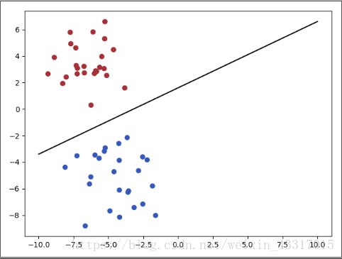
而分类,则是要把结果进行区分,如下图:
我们可以很容易的找到一条线性的分类器(直线)来将红色和蓝色的点区分开来;
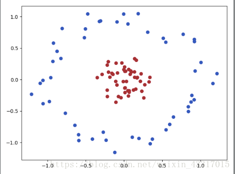
但是现实中,很多问题并不能用线性的关系来进行分类,如下图,
线性的分类肯定不能将红蓝两部分完全分开,需要采用非线性的分类器来对这样的两类进行分类。
这里看上去和逻辑回归并没有关系。但是如果我们想知道对于一个二分类问题,我们不仅想知道该类属于某一类,而且还想知道该类属于某一类的概率多大,有什么办法呢?
这样我们就需要采用逻辑回归来达到我们的目标,也就是逻辑回归,实际上是解决二分类问题的算法。
二、sigmoid 函数
这里的问题,我们可以理解成图2中的任意一点,都是需要我们对其进行判断的 ,而目标 就是属于某一类的概率;
而一般线性的分类表达式为:
这里的
,而对于目标概率值,我们会希望
,所以我们首先需要将
预测的概率映射到
,而sigmoid函数可以帮助我们实现这一操作;
sigmoid 函数工式:
sigmoid 函数图像显示如下:
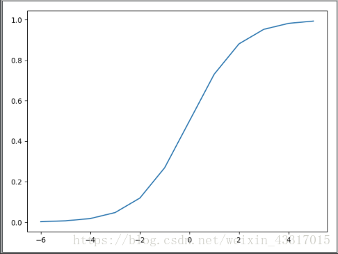
这样就可以让 ,对应映射到 ,当 时, 。
三、建立目标函数
有了sigmoid函数,我们可以将目标函数由原来的
,可以带入sigmoid函数中,那么目标函数为:
因为现在是个分类任务,那么
对应的概率则为:
这样我们又将问题转换为,要
的值越大预测值越接近真实值;沿用前述的求概率最大值的方法,接下来我们要引用似然函数来进行累乘再转换为对数似然函数,转成累加来解决这个问题;
四、似然函数(对数似然)求极值
下面我们就来用似然函数(对数似然),来对目标函数的
值来进行求极值;
转换为对数似然:
上式我们要求最大值,可以用代数的性质转变一下,前面加任意负的常数(
)来求最小值,将这个问题转换为梯度下降来求解;
对
将目标函数
带入上式,并对
展开求导:
求导的结果是:
所以我们可以将 带入求导,后再换成
下面就省略详细的求导过程,步骤如下:
五、逻辑回归(Logistic Regression)
参数更新:
多分类器的softmax:
- 总结
优点:
1、实现起来比较方便且简单;
2、训练时计算较快,消耗资源较小;
缺点:
1、只能处理必须线性可分的问题;
2、一般准确度不太高;
六、Python代码实现
使用sklearn模块中的线性回归算法的代码:
import numpy as np
import pandas as pd
from sklearn import linear_model
import matplotlib.pyplot as plt
from sklearn.model_selection import cross_val_predict,KFold,train_test_split
from sklearn.linear_model import LogisticRegression
#传入需要进行预测的数据
loans = pd.read_csv('./data/cleaned_loans2007.csv')
#实例化算法
lr = LogisticRegression(class_weight='balanced')
train,test = train_test_split(loans,test_size=0.3)
#对模型进行训练
lr.fit(train.loc[:,train.columns !='loan_status'],train['loan_status'])
#输出预测值
predict = lr.predict(train.loc[:,train.columns !='loan_status'])
predict = pd.Series(predict)
#通过False positive rate(FPR)以及True positive rate(TPR)进行判断模型是否可行
fp = (predict==0)& (train['loan_status'] ==1)
tp = (predict==0)& (train['loan_status'] ==0)
fn = (predict==1)& (train['loan_status'] ==0)
tn = (predict==1)& (train['loan_status'] ==1)

FPR = fp.sum()/(fp.sum()+tn.sum())
TPR = tp.sum()/(tp.sum()+fn.sum())
print(FPR,TPR)
不使用已有算法方法,来写线性回归算法的代码,实例:
数据为以两门学科成绩,预测是否会录取
#coding=utf-8
# write by sz
import matplotlib
import numpy as np
import pandas as pd
import  matplotlib.pyplot as plt
# %matplotlib inline
import  time
import os


# print(os.path.dirname(__file__))
path =os.path.dirname(__file__) + os.sep + 'LogiReg_data.txt'
data = pd.read_csv(path,header=None,names=['EXAM 1','EXAM 2','ADMITTED'])
print(data['EXAM 1'].shape,data['ADMITTED'].shape)
postive = data[data['ADMITTED'] == 1]
negtive = data[data['ADMITTED'] == 0]

'''
画图展示样本数据
 plt.scatter('EXAM 1','EXAM 2',s=30,c = 'r',marker='x',data=postive,label='admitted')
 plt.scatter('EXAM 1','EXAM 2',s=30,c = 'y',marker='^',data=negtive,label='unadmitted')
 plt.legend(loc='best')
 plt.show()
'''
'''
SIGMOID 函数
'''
def sigmoid(x):

    return 1/(1+np.exp(-x))

'''
model 模块
'''
#model 函数
def model(X,theta):
    # x=X.dot(theta.T)
    x = np.dot(X,theta.T)
    # print(x)

    return sigmoid(x)

'''
COST 函数
'''
def cost(X,theta,y):

    left = np.multiply(-y,np.log(model(X,theta)))
    right = np.multiply((1-y),np.log(1-model(X,theta)))
    # left= np.log(model(X,theta))
    # right = -y
  return np.sum(left-right)/(len(X))


'''
梯度计算
'''
def gradient(X,y,theta):

    error = (model(X,theta)-y).ravel()
    # error1 = (model(X, theta) - y)

    grad = np.zeros(theta.shape)
    # grad1 = np.zeros(theta.shape)

    for j in  range(theta.shape[1]):

        # gr = np.dot(X[:,j],error1)
        gr = np.multiply(error, X[:, j])

        grad[0,j] = np.sum(gr)/len(error)
        # grad1[0, j] = np.sum(gr1) / len(X)

    return grad


'''
定义梯度下降停止方式
'''
stop_by_iter = 0
stop_by_cost = 1
stop_by_grad = 2

def stop(types,value,target):

    if types == 0 :
        if value%100==0:
            print(value)
        return value > target

    elif types == 1:
        return value[-1] < target

    elif types == 2:
        return np.linalg.norm(value) < target

'''
清洗数据(洗牌)
'''

def shuffle(data):

    np.random.shuffle(data)

    cols = data.shape[1]
    X = data[:,0:cols-1]
    y = data[:,cols-1:cols]

    return X,y

'''
梯度下降更新计算
'''
def descent(data,alpha,theta,bathsize,stoptype,target):
    in_time = time.time()
    k = 0
    X,y = shuffle(data)
    costs = [cost(X,theta,y)]
    i = 0
    n = len(X)
    while True :
        grad = gradient(X[k:k+bathsize],y[k:k+bathsize],theta)
        k += bathsize
        if k > n:
            k = 0
            X,y = shuffle(data)
        theta = theta - alpha * grad
        costs.append(cost(X,theta,y))
        i +=1
        if stoptype == 0:
            value = i
        elif stoptype == 1:
            value = costs
        elif stoptype == 2:
            value = grad
        if stop(stoptype,value,target):
            break

    return theta,costs,grad,i,time.time()-in_time

'''
结果可视化展示
'''
def plant(i,costs):
    # plt.plot(np.arange(i+1),costs,'b')
    # plt.figure(figsize=(12,4))
    fig, ax= plt.subplots()
    ax.plot(np.arange(i+1),costs,'b')
    ax.set_ylim(0,3)
    # plt.xlim(0,i)
    # plt.ylabel('cost')
    # plt.xlabel('iteration')
    plt.show()


'''
计算精度
'''
def predict(X,y,theta):

    result=[]

    for i in range(len(X)):

        if model(X[i,:],theta) > 0.7 :
            result.append(1)
        else:
            result.append(0)
    percent=(y.ravel() == result).sum()/len(y)*100

    return percent
if __name__ =='__main__':
#数据处理
theta = np.zeros([1,data.shape[1]])

data.insert(0,'X0',value=1)

pdate  = data.values
cols = data.shape[1]
#
X = pdate[:,0:cols-1]

# y = pdate[:,cols-1]
y = pdate[:,cols-1:cols]
'''
以不同梯度下降方式停止:
theta,costs,grad,i, dua = descent(pdate,0.001,theta,16,stop_by_iter,1000000)
'''
theta,costs,grad,i, dua = descent(pdate,0.001,theta,8,stop_by_grad,0.005)

plant(i,costs)
#print(costs[-1])
#print(theta)
#print(dua)

re=predict(X,y,theta)

print('精准度为:%d%%' %re)
以上,就是本次学习的逻辑回归的数学推导,以及python代码实现的案例;